MetX Example Dashboard - Agriculture

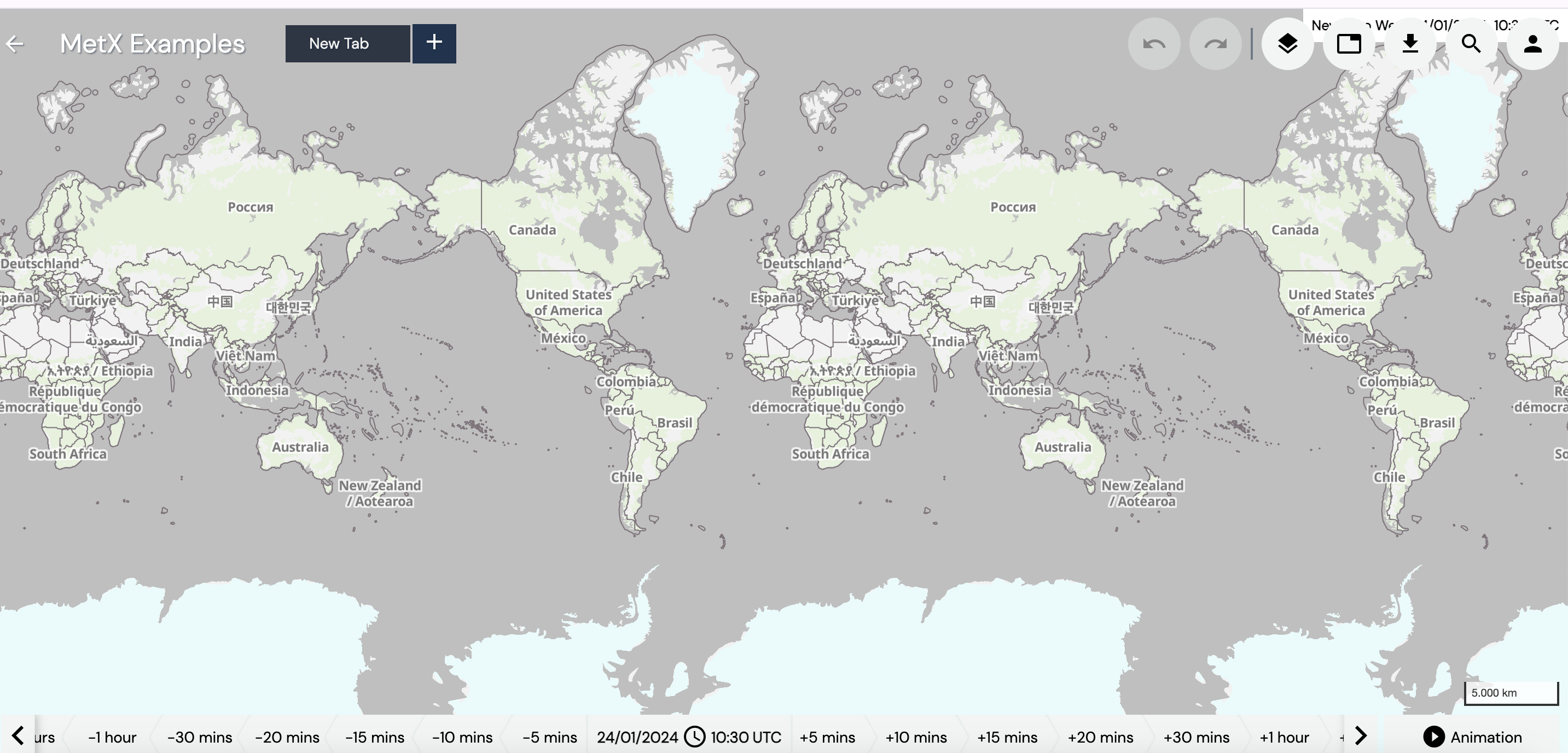
In our third example, we create an agricultural map. You can use the dashboard from the previous examples (Weather overview or Aviation) and open a new tab by clicking on and clicking the ”Add Map” icon or you can create a new dashboard in the welcome screen (see section First Navigation). To create a new dashboard, click on the ”Create Dashboard” button, enter the name of your new dashboard e.g. ”MetX Examples” and click on the ”Apply” button. In both cases, your screen looks now similar to the following:

Now, the newly created tab can be renamed e.g. with ”Agriculture” by clicking on ”New Tab”.
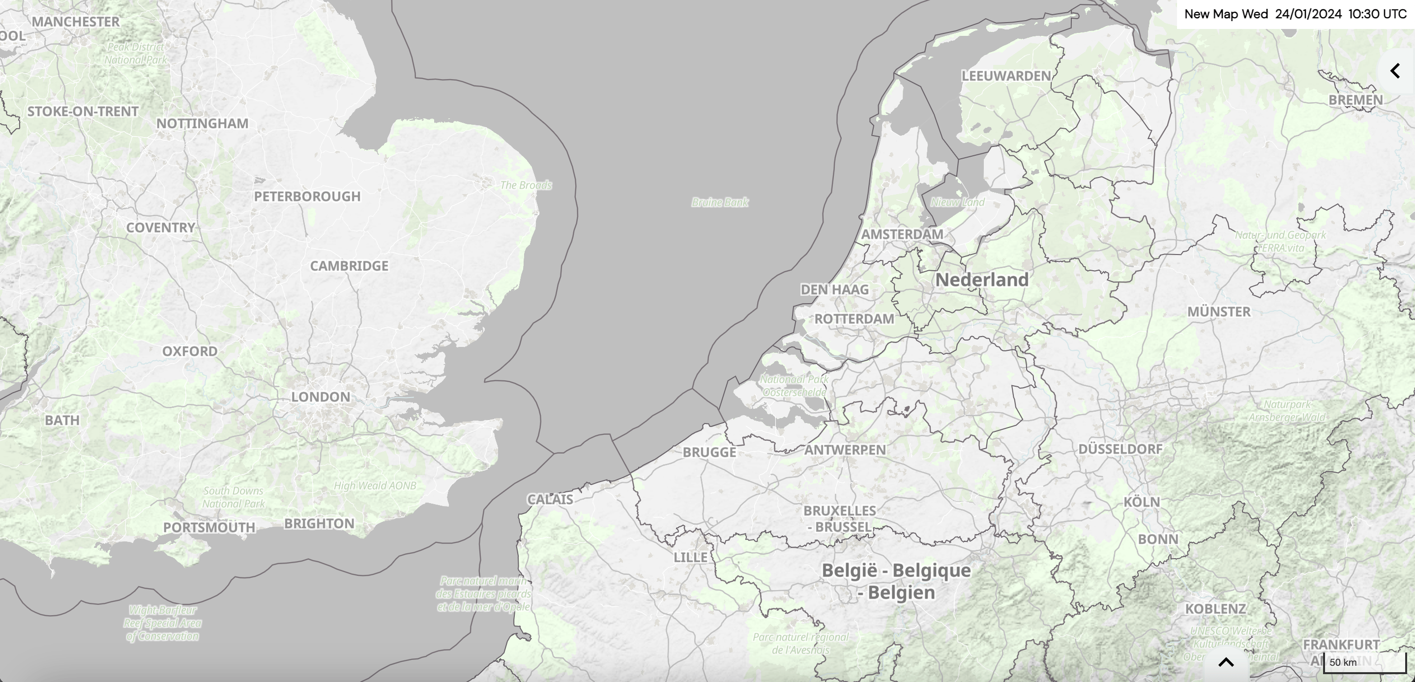
To have a closer look at a certain region, you can zoom in e.g. to the Netherlands. Press and hold the left mouse button to change the map extent and scrolling in and out controls the level of zooming into the map.

We want to add parameters on four parallel maps. Click on to change the general tab settings. Click the option at the top to get four maps next to each other. Set the ”MAP SYNC” to ”On” and click the ”Add Map” icon for the map at the bottom left, and for the two maps on the right click on the ”Add Plot” button.

In a next step, select the desired parameters. Click on to open the Layer Stack.

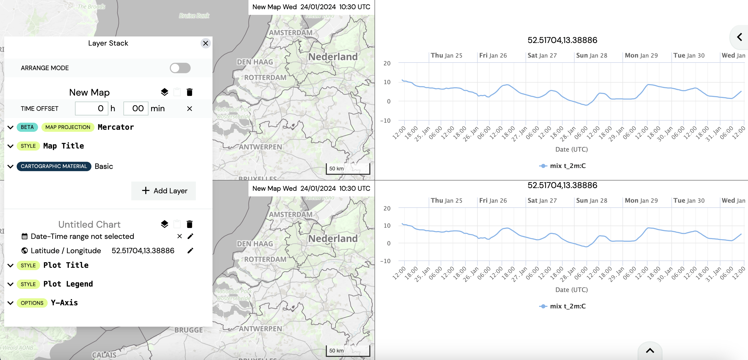
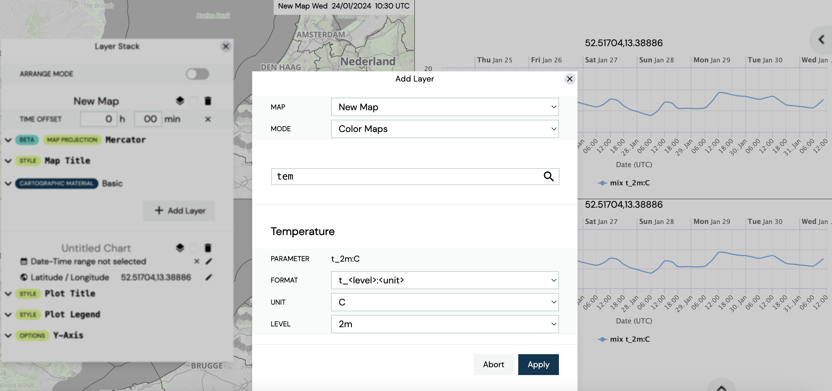
The stack at the top shows the parameter layers for the map in the top left corner (you can check that by moving the cursor over the respective parameter layers - a turquoise frame appears on the map or plot you are working on), the second stack the ones for the map in the lower left corner, the third stack the ones for the map in the top right corner and the last stack shows the parameter layers for the map in the lower right corner (however, this order might vary as it depends on the order in which the maps were added). Click the ”Add Layer” button on the bottom right of the Layer Stack of the first map in the upper left corner. A new window opens. Select ”Color Maps” as ”MODE” and type ”t” in the ”Search for weather parameters”. Click on ”Temperature” at the very top of the suggested parameters.

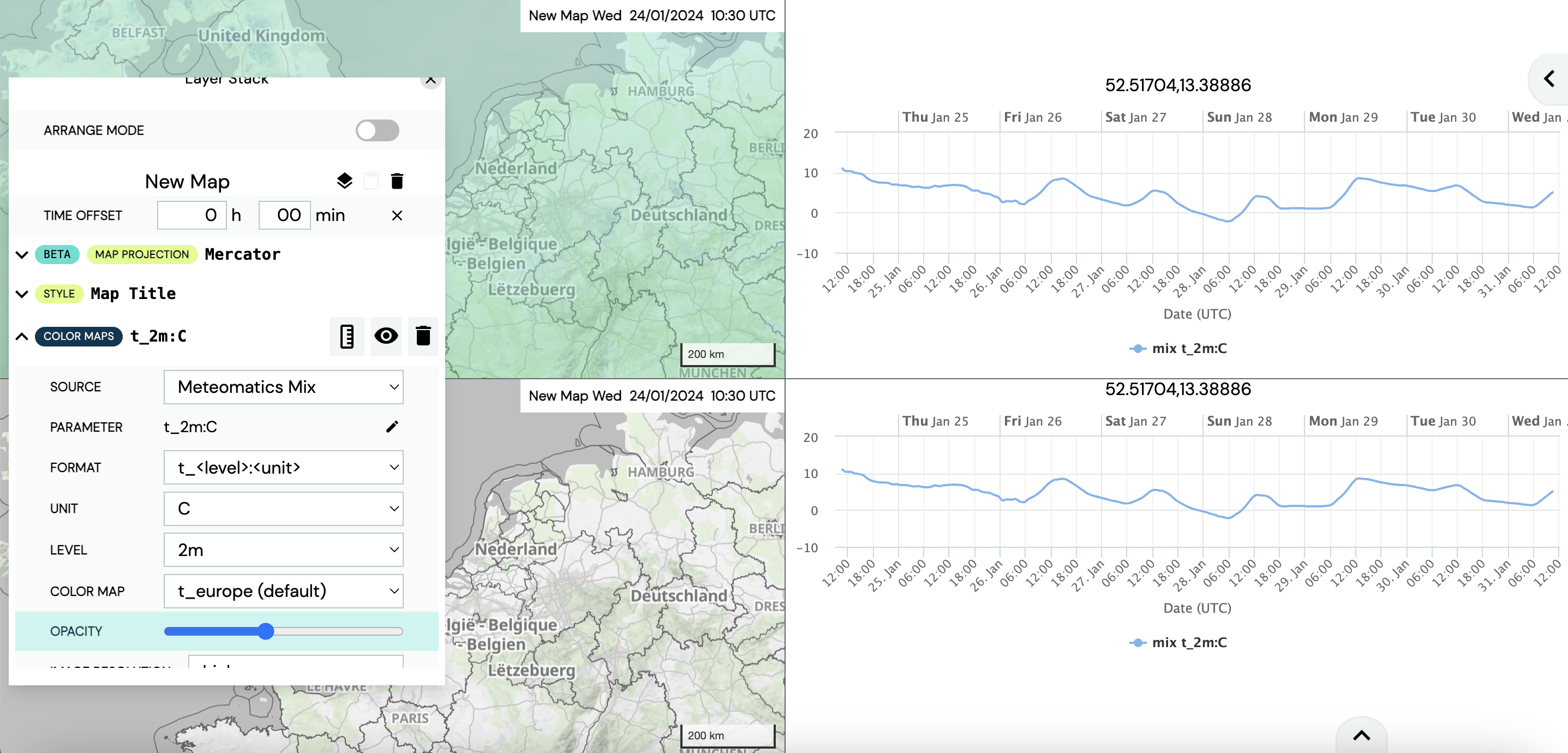
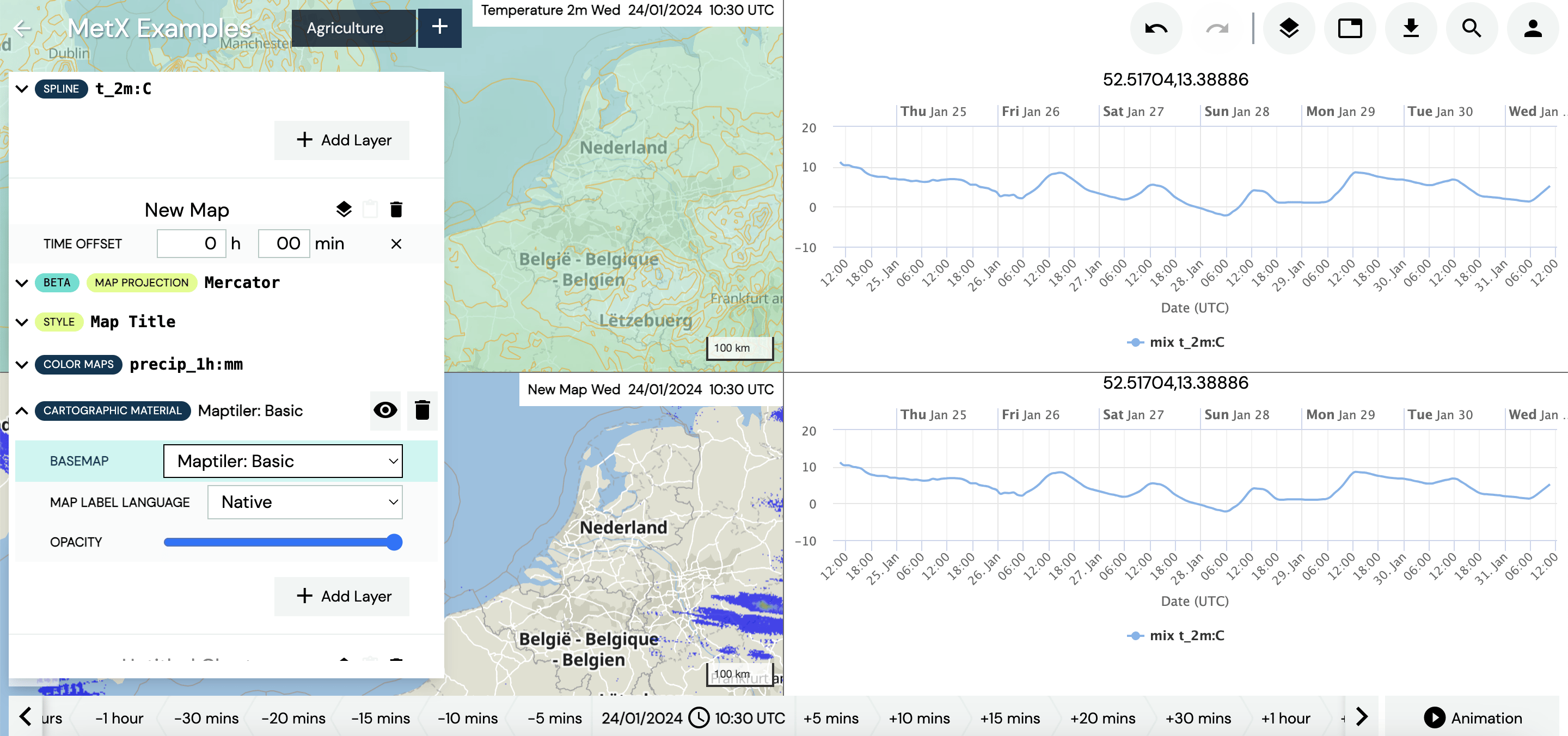
If desired, the user can change the preferences of the temperature by clicking on ”COLOR MAPS t_2m:C” on the Layer Stack (see section Colour Maps). In this example, we decrease the ”OPACITY” a bit (move the slider slightly to the left hand side). For the rest, we keep the default values.

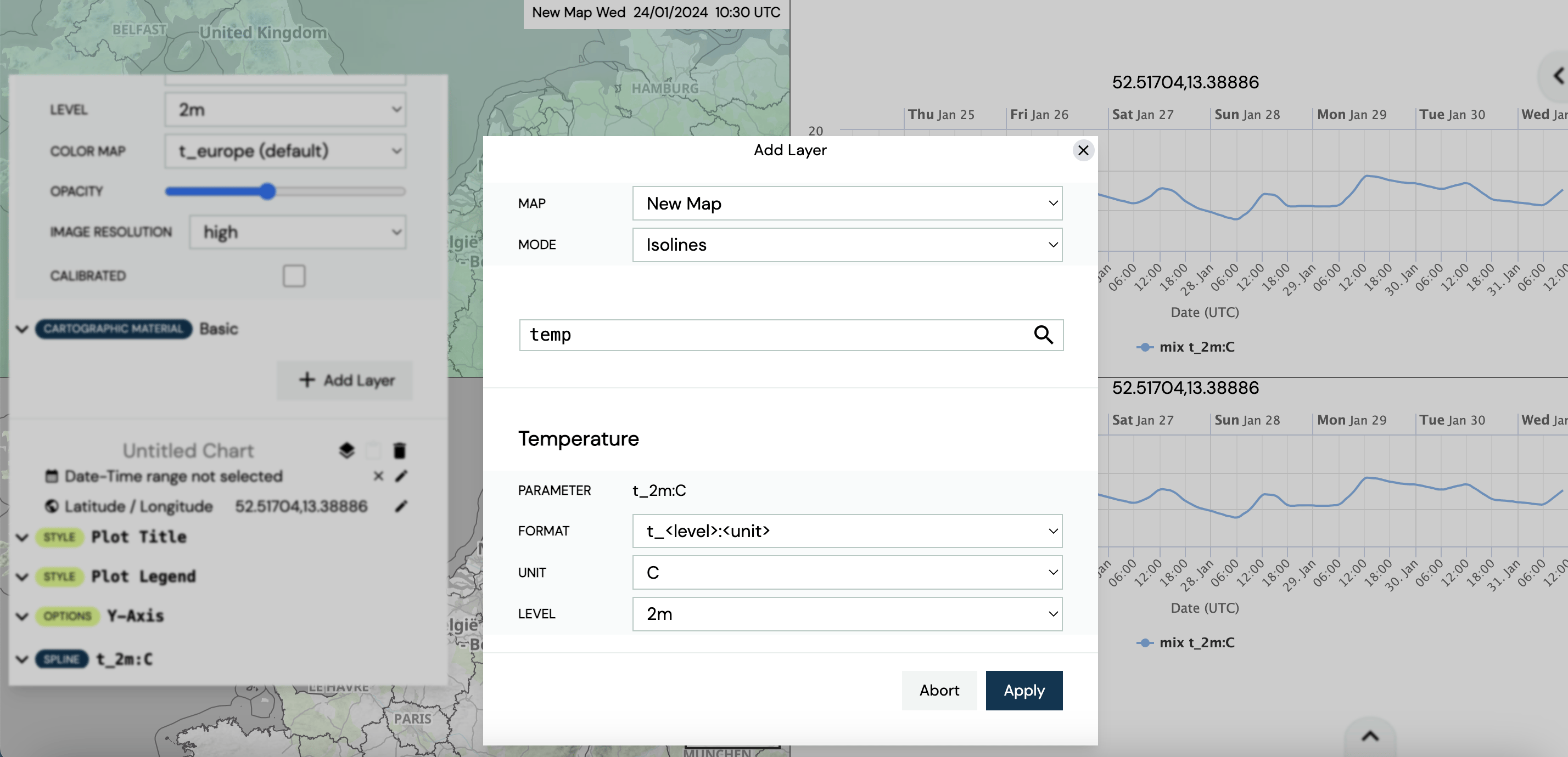
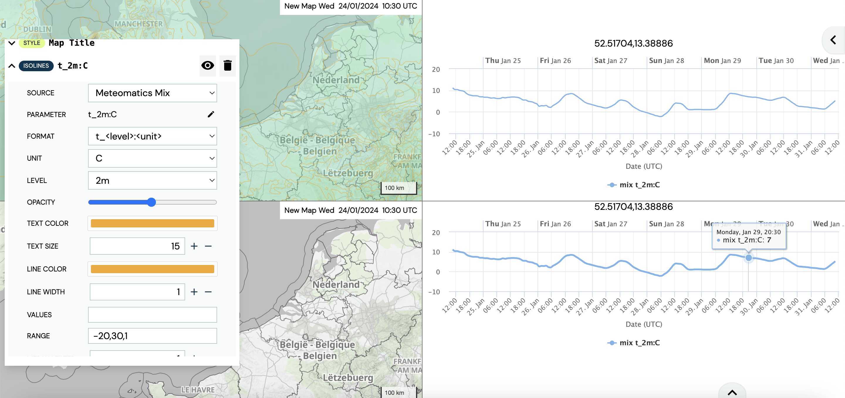
In a next step, we add the isolines of the 2 meter temperature to the first map in the upper left corner. Click on the ”Add Layer” button on the bottom right of the Layer Stack of the first map. Select ”Isolines” as ”MODE” and type ”t” in the ”Search for weather parameters” box to add temperature isolines to the map (see section Isolines). Select the parameter ”Temperature” at the very top by clicking on it and specify afterwards the parameter properties (format, unit and level).

To change the preferences for temperature isolines, click on the Layer Stack on ”ISOLINES msl_pressure:hPa”. In this example, we decrease the ”OPACITY” a bit (move the slider slightly to the left hand side). Further- more, we change the ”TEXT COLOR” and ”LINE COLOR” to orange-red, the ”TEXT SIZE” to 15 and add a ”RANGE”. For the minimum value we insert -20 °Celsius and for the maximum 30 °Celsius using a step of 1 °Celsius (see also section Isolines). For the rest, we keep the default values.

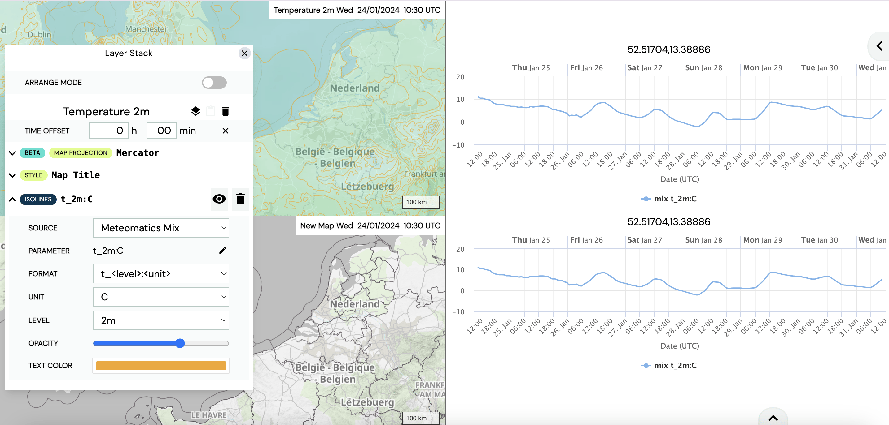
To change the underlying cartographic map, click on the Layer Stack on ”CARTOGRAPHIC MATERIAL Ba-sic” and select a ”BASEMAP” (see section Cartographic Material). In this example, we choose the ”Maptiler:Basic” as ”BASEMAP”.
As a last step, we change the title of the first map by clicking on ”New Map” on the Layer Stack and typing e.g. ”Temperature 2m” in the box. Click the ”STYLE Map Title” on the Layer Stack to adapt the design of the title (see section Map title design). In this example, we keep the default setting.

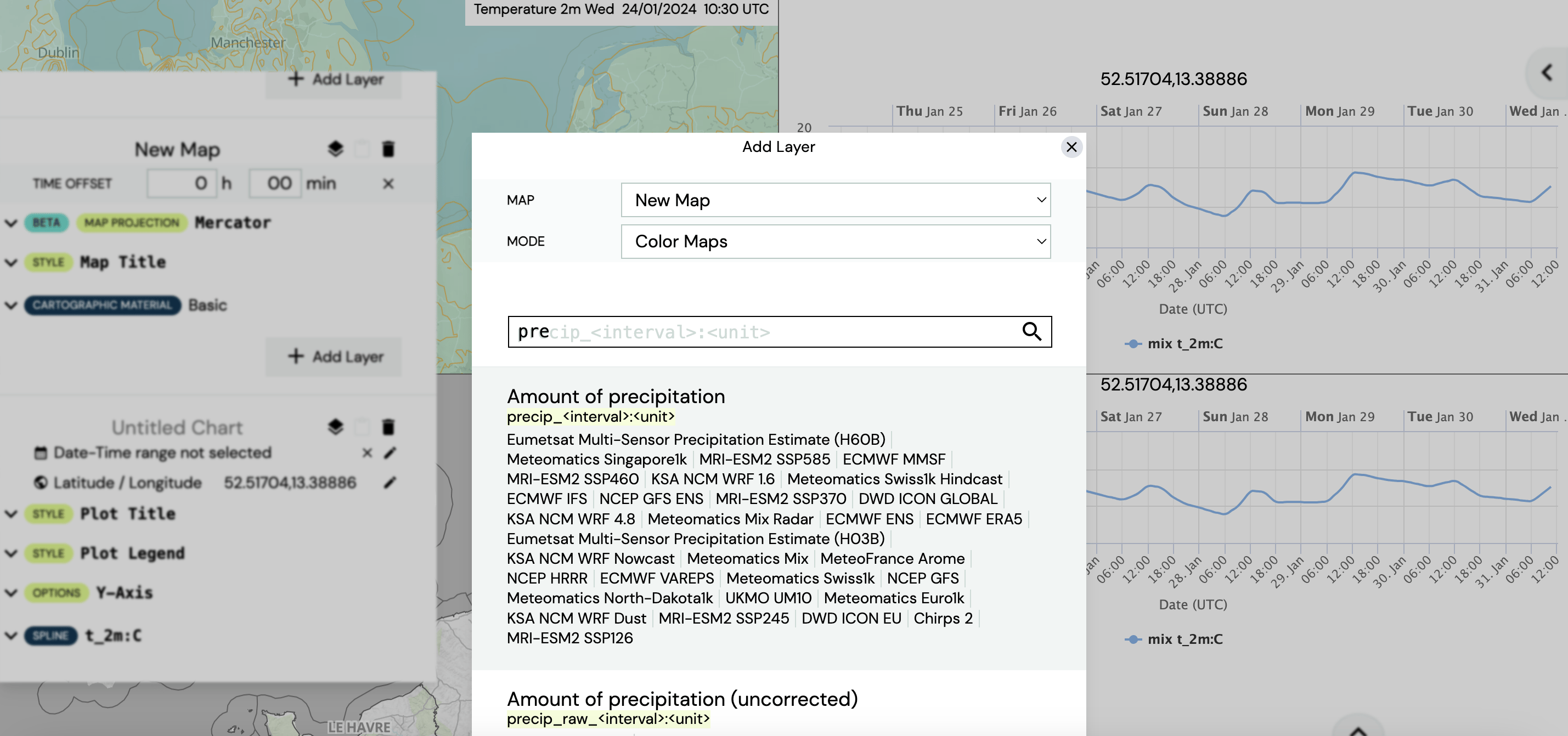
Next, we want to set up the second map on the lower left side. Click on the ”Add Layer” button on the bottom right of the Layer Stack of the second map. We want to add a new colormap. Thus, select ”Color Maps” as ”MODE” (see section Colour Maps). Then, type ”precip” in the ”Search for weather parameters” box to add precipitation to the map. Select the parameter ”Amount of precipitation” at the very top by clicking on it.

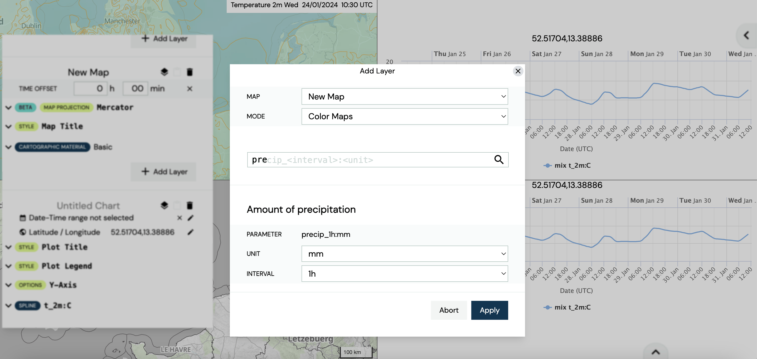
Now, you can specify the parameter properties (format, unit and interval). In this example, we choose for the precipitation the format ”precip_<interval>:<unit>”, the unit ”mm” and an interval of 1 hour. Thus, the amount of precipitation in the previous hour in mm is displayed after clicking the ”Apply” button.

The user can change the colormap’s preferences by clicking on ”COLOR MAPS precip_1h:mm” on the Layer Stack (see section Colour Maps). In this example, we stick to the default values.
To change the underlying cartographic map, click on the Layer Stack on ”CARTOGRAPHIC MATERIAL Ba- sic” and select a ”BASEMAP” (see section Cartographic Material). In this example, we choose the ”Map- tiler:Basic” as ”BASEMAP”.

As a last step, we change the title of the second map by clicking on ”New Map” on the Layer Stack and typing e.g. ”Precipitation” in the box. Click the ”STYLE Map Title” on the Layer Stack to adapt the design of the title (see section Map title design). In this example, we keep the default setting.
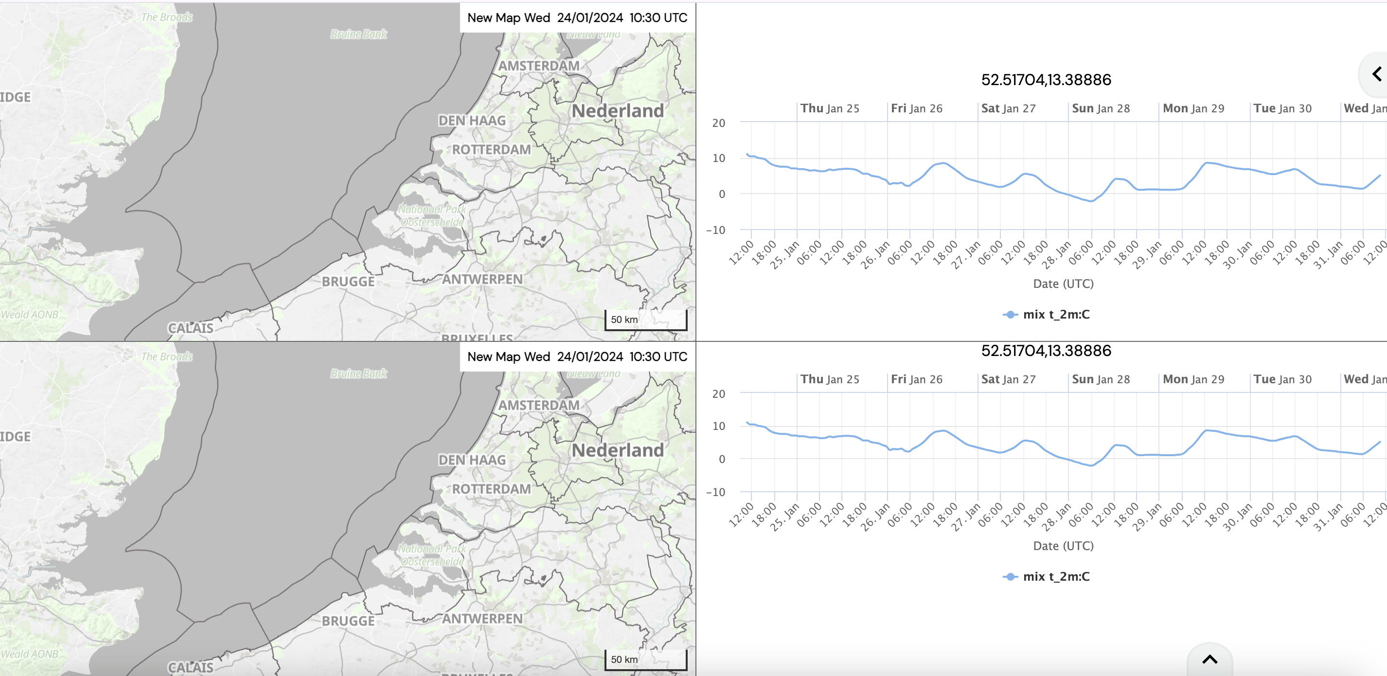
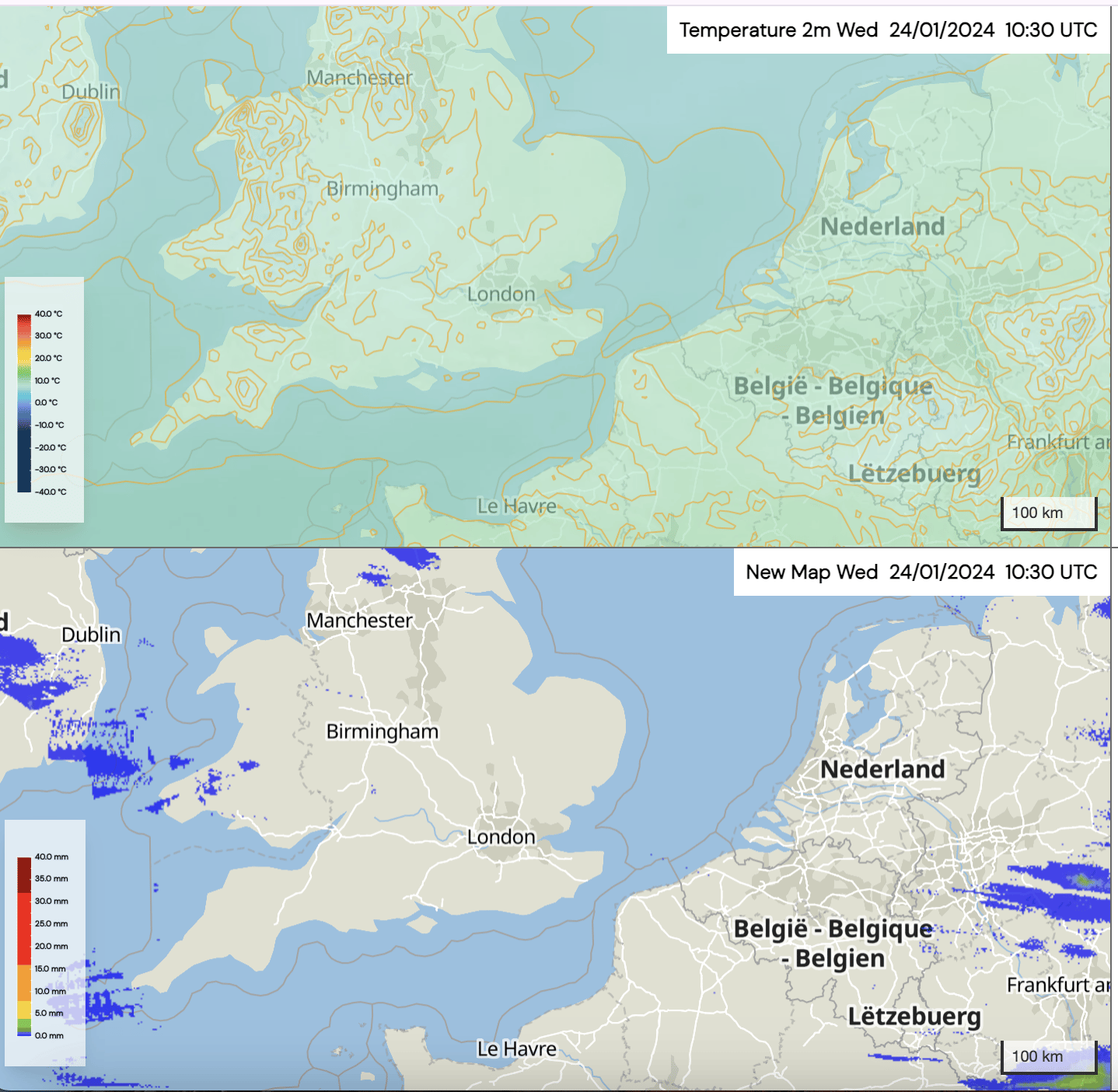
Your final two maps on the left hand side look now similar to the following:

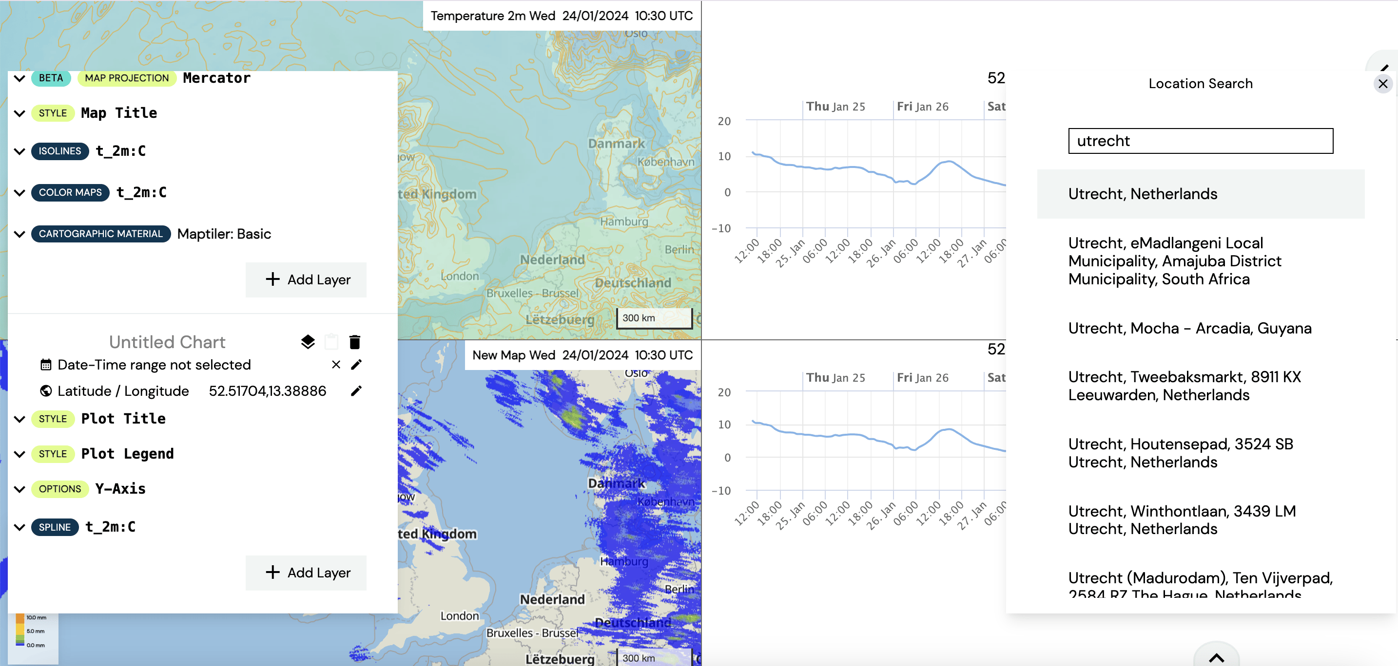
In a further step, we set up the plot on the upper right side (see section Plots in MetX). First, click on the little pencil next to the ”Latitude / Longitude” section of the third map (in this case the one below the Precipitation) on the Layer Stack. A window called ”Location Search” at the upper right side of the map appears. Specify in the ”Search” field the desired coordinate. We want to investigate Utrecht in the Netherlands and thus type Utrecht in the ”Search” box and click on the first suggestion.

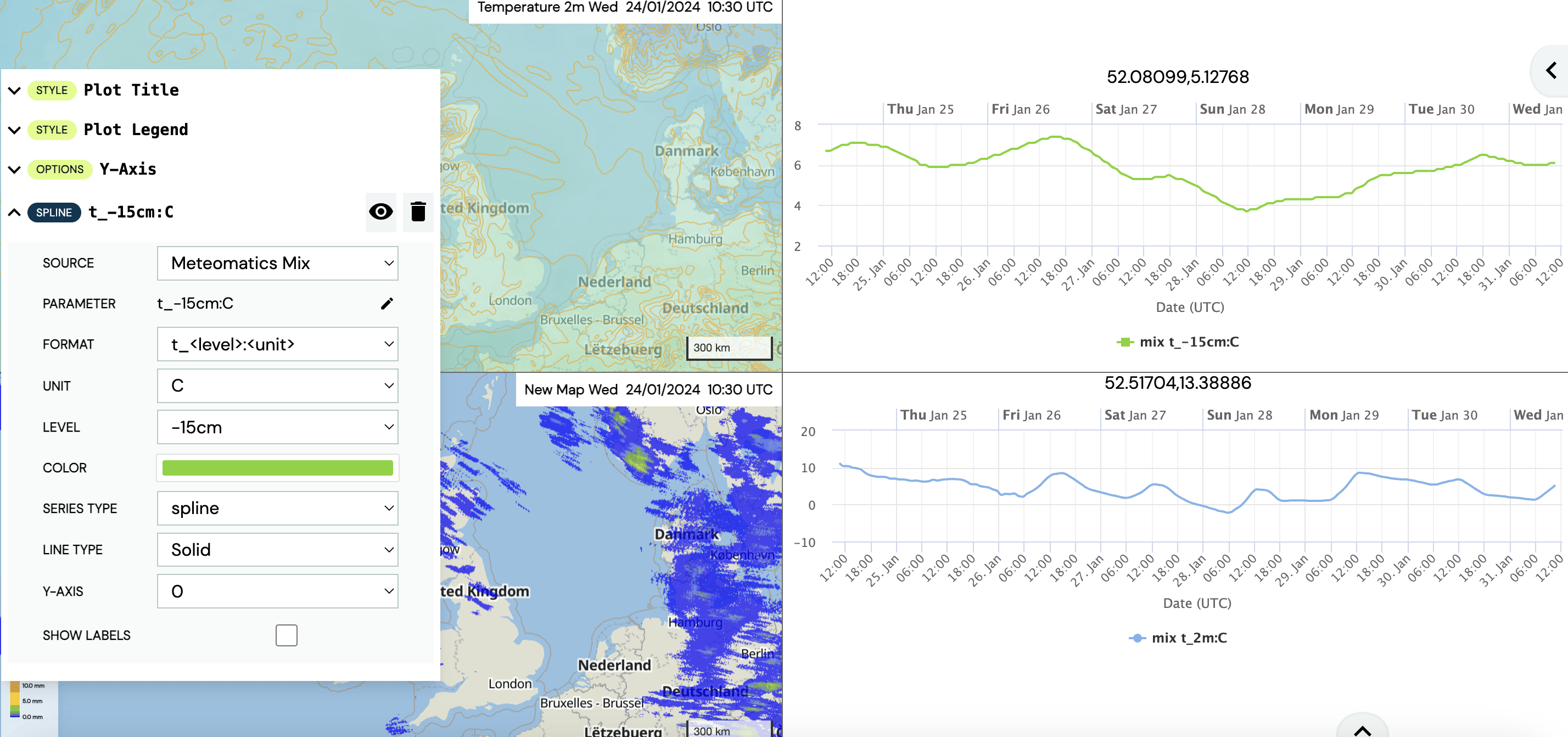
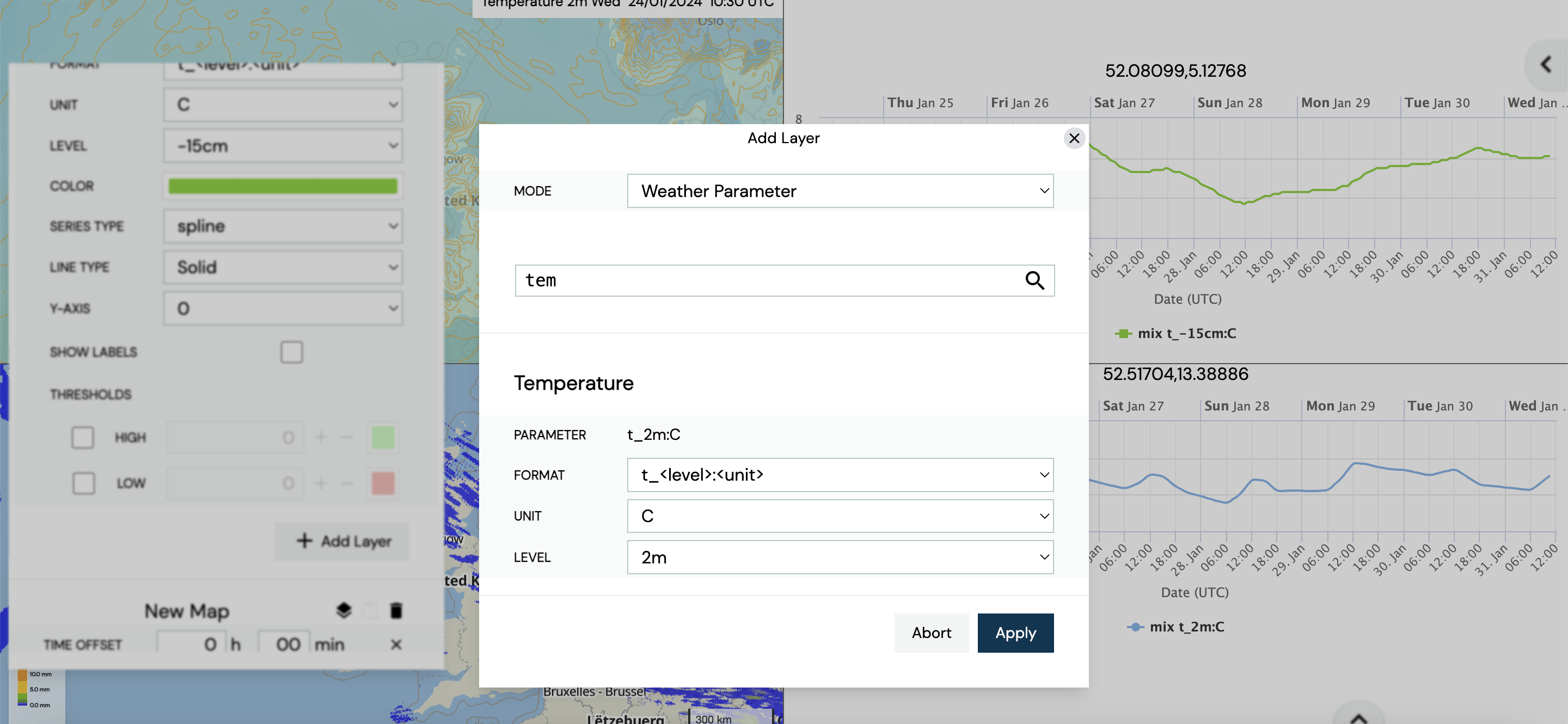
Now, we want to add several temperature timeseries on the plot. As default, there is already the 2 meter temperature displayed on the map. We change this parameter into the -15cm temperature. Click on ”SPLINE t_2m:C” on the Layer Stack. Change the ”LEVEL” to -15cm and the ”COLOR” to green.

Let’s add the minimum, maximum and the 10 year mean 2m temperature to the plot. Click on the ”Add Layer” button on the bottom right of the Layer Stack. Type ”t” in the ”Search for weather parameters” box and click on the first suggestion:

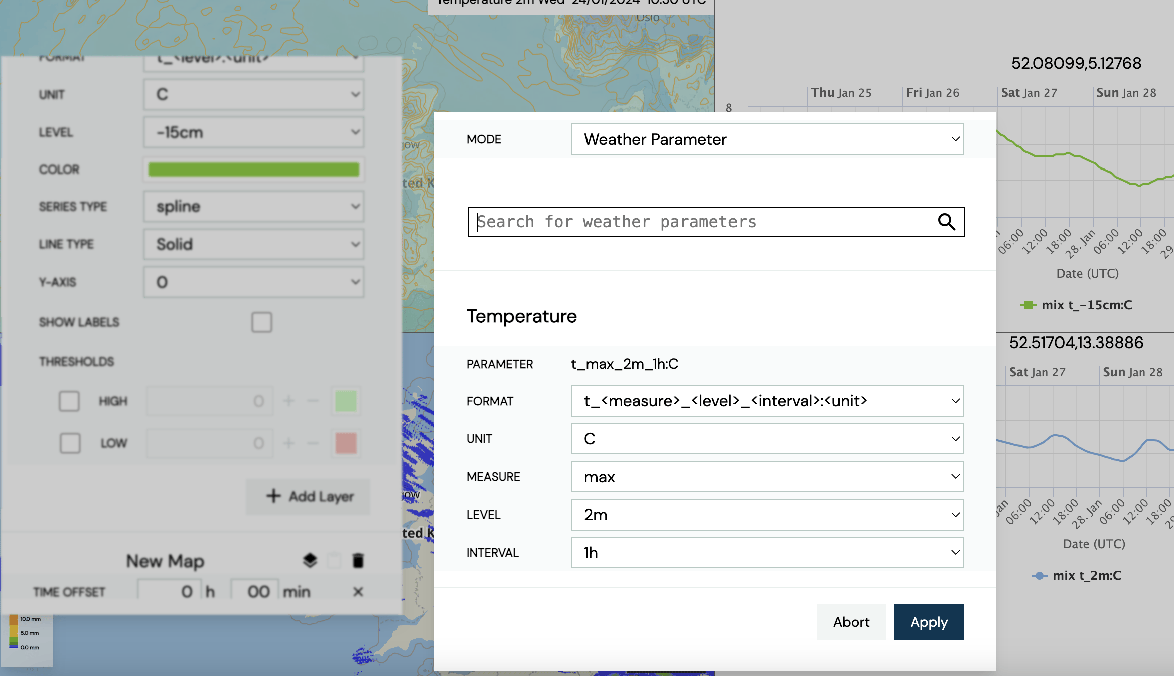
Now, you can specify the parameter properties (format, unit, measure, level and interval). In this example, we choose the format ”t_<measure>_<level>_<interval>:<unit>”, the unit ”C”, the measure ”max”, the level ”2m” and an interval of 1 hour. Thus, the maximum temperature 2 meters above the ground in the previous hour is displayed after clicking the ”Apply” button.

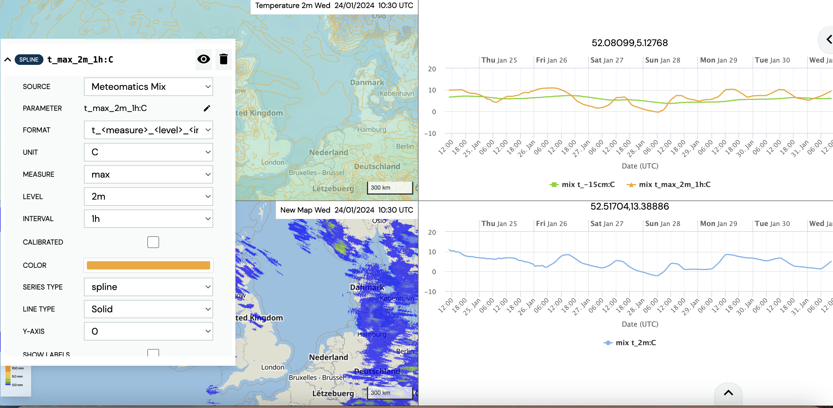
Change the preference of the newly added maximum temperature by clicking on ”SPLINE t_max_2m_1h:C” on the Layer Stack. We change the ”COLOR” to orange and keep the rest as it is.

Next, we add the 10 year mean 2m temperature by clicking on the ”Add Layer” button on the bottom right of the Layer Stack. Type ”t” in the ”Search for weather parameters” box and click on the first suggestion.

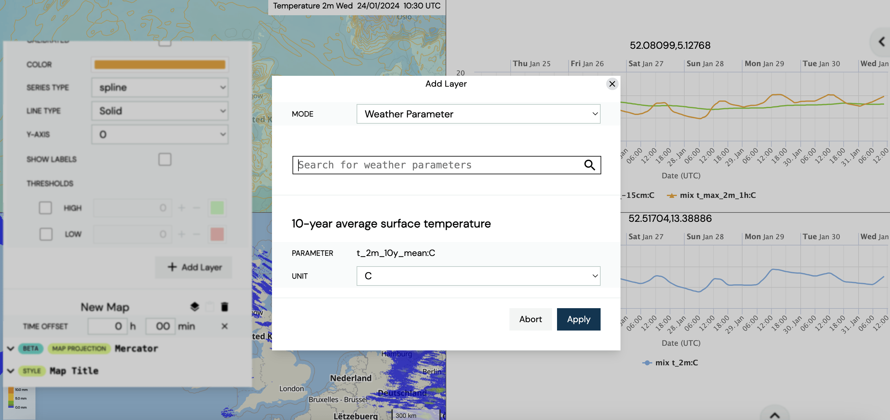
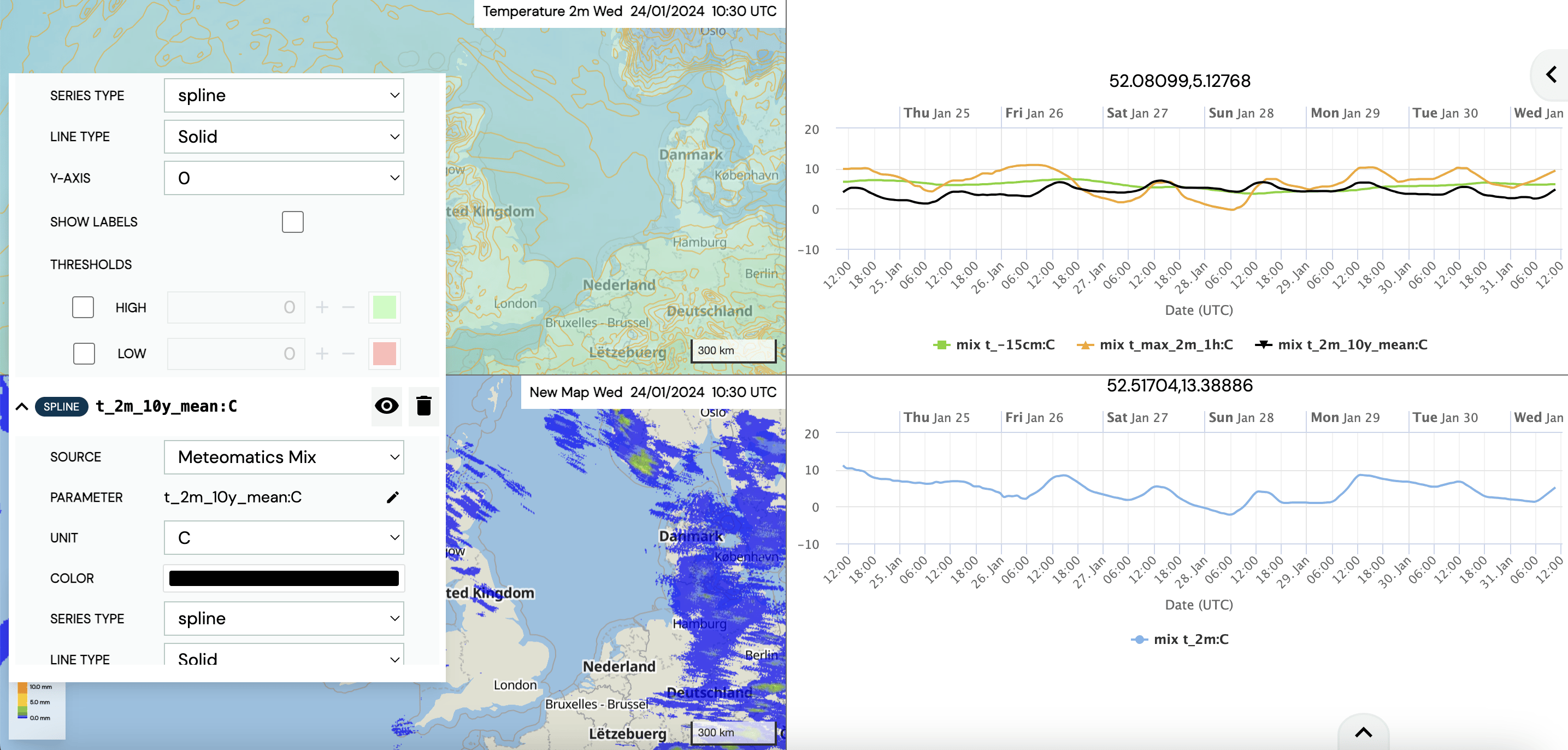
Change the preference of the newly added 10 year temperature by clicking on ”SPLINE t_2m_10y_mean:C” on the Layer Stack. We change the ”COLOR” to black and keep the rest as it is.

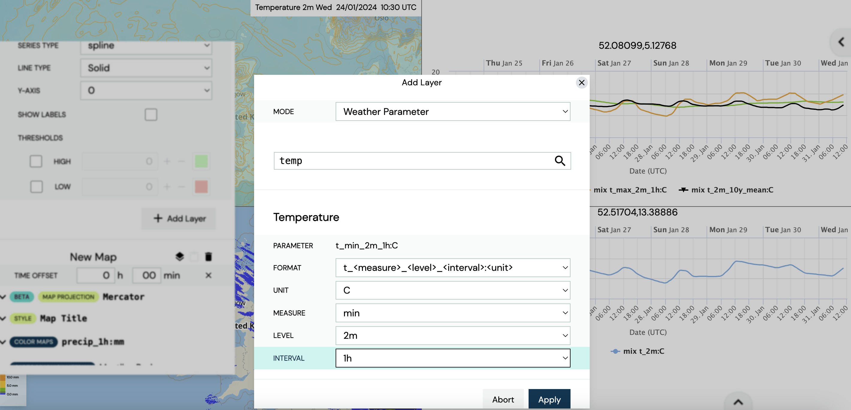
Finally, we add the minimum 2 meter temperature to the plot by clicking on the ”Add Layer” button on the bottom right of the Layer Stack. Type ”t” in the ”Search for weather parameters” box and click on the first suggestion.
Now, you can specify the parameter properties (format, unit, measure, level and interval). In this example, we choose the format ”t_<measure>_<level>_<interval>:<unit>”, the unit ”C”, the measure ”min”, the level ”2m” and an interval of 1 hour. Thus, the minimum temperature 2 meters above the ground in the previous hour is displayed after clicking the ”Apply” button.

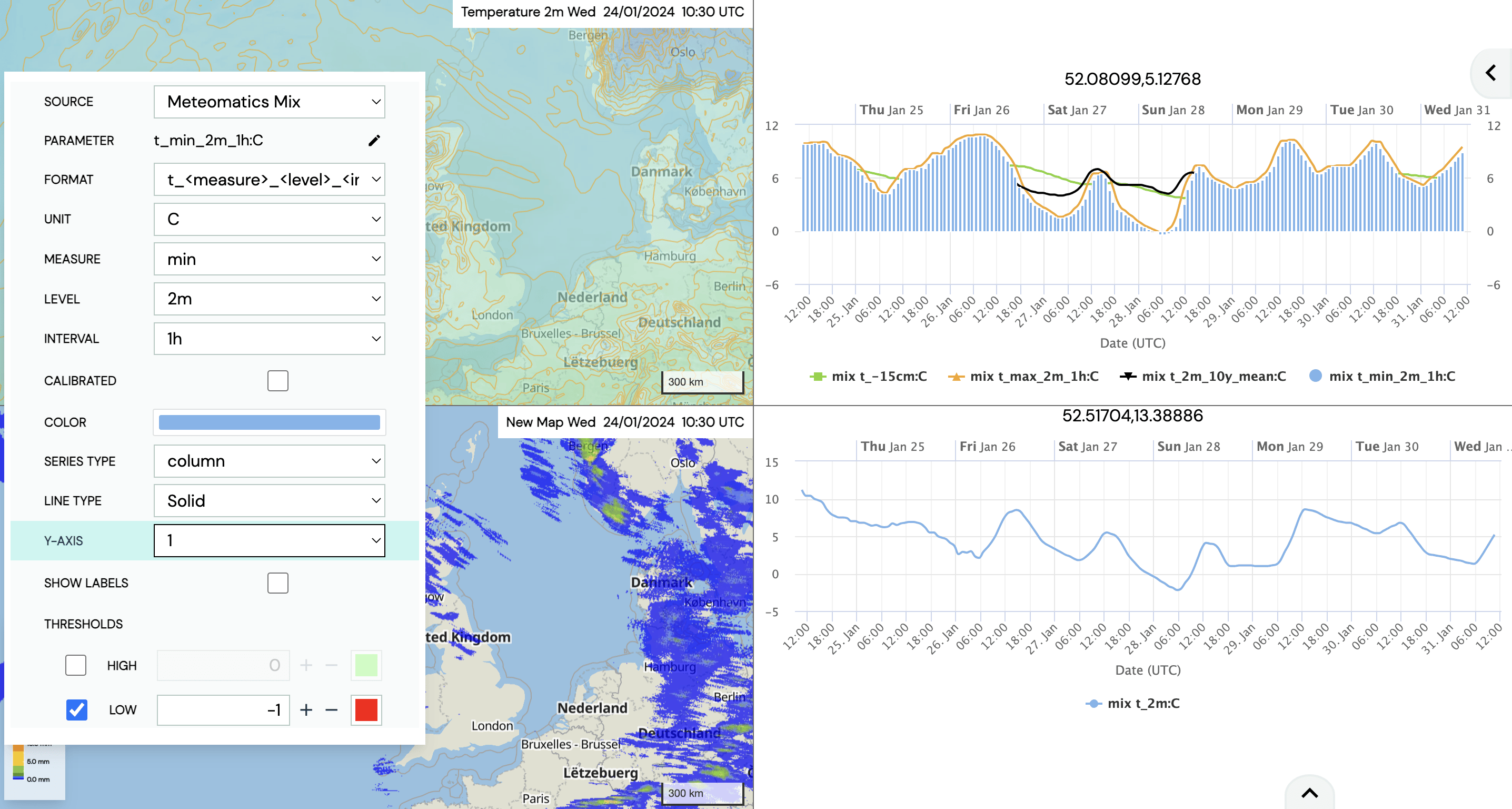
Change the preference of the newly added minimum temperature by clicking on ”SPLINE t_min_2m_1h:C” on the Layer Stack. We change the ”COLOR” to blue, the ”SERIES TYPE” to ”column”, the ”Y-AXIS” to 1, check the ”LOW” box in the ”THRESHOLDS” section and set the value to -1. For the rest, we keep the default setting.

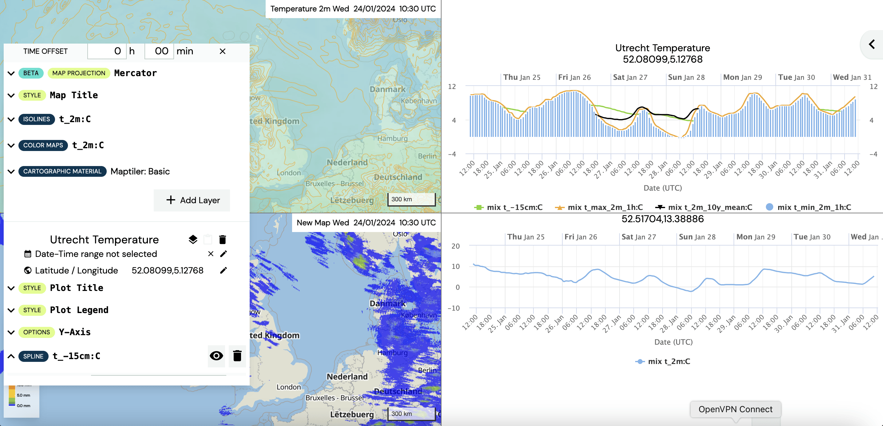
In our last step, we change the title of the plot. Click on ”Untitled Chart” on the Layer Stack and type e.g. ”Utrecht Temperature” in the box. Click the ”STYLE Plot Title” on the Layer Stack to adapt the design of the title. In this example, we change the font size to 20 and check the ”bold” box. Also, you can change the design of the legend by clicking on ”STYLE Plot Legend” on the Layer Stack. In this example, we keep the default setting.

Now, let’s create our last plot on the lower right side. Again, change the coordinate by clicking on the little pencil next to the ”Latitude / Longitude” section of the fourth map (in this case the one at the bottom) on the Layer Stack. A window called ”Location Search” at the upper right side of the map appears. Specify in the ”Search” field the desired coordinate. We still want to investigate Utrecht in the Netherlands and thus type Utrecht in the ”Search” box and click on the first suggestion.
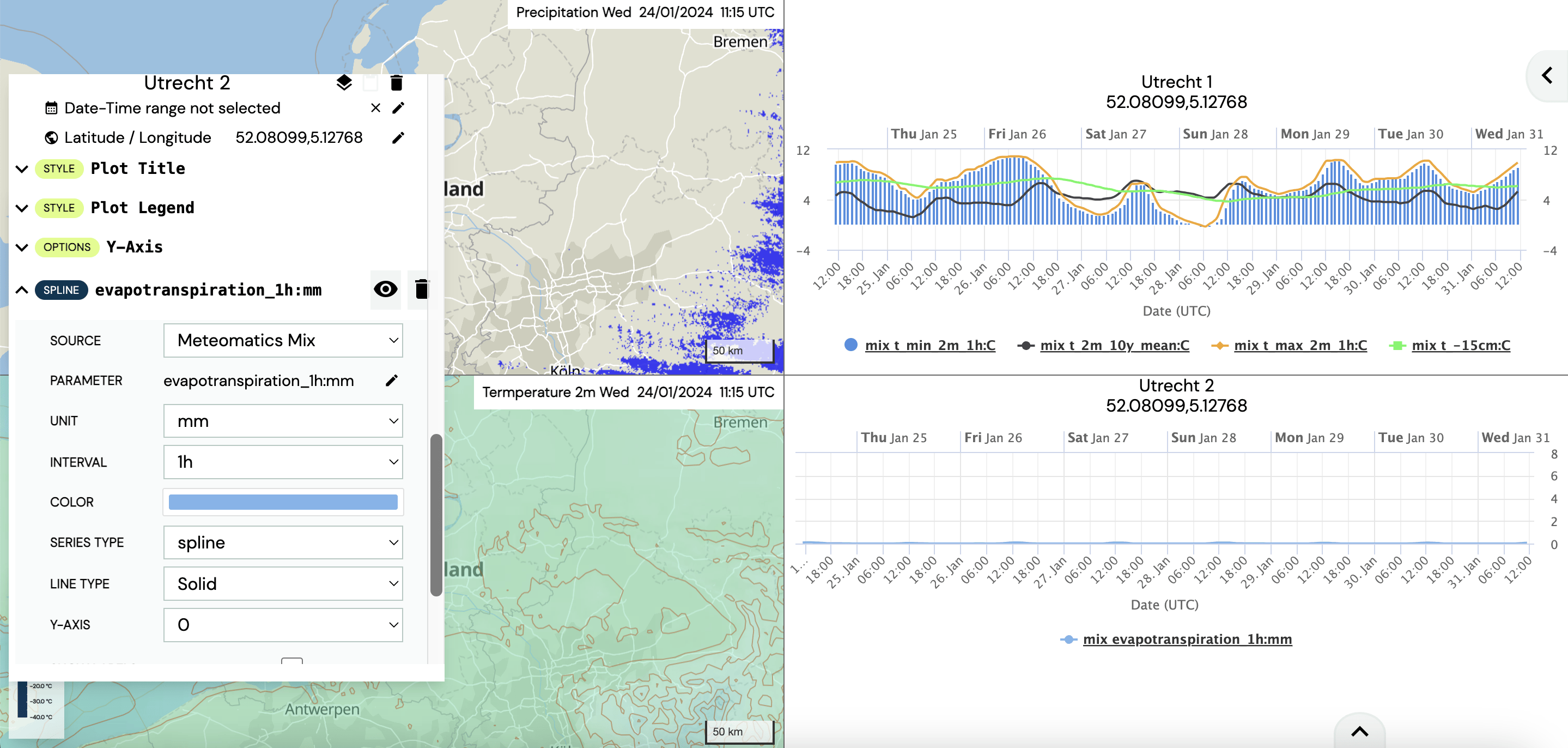
As default, there is already the 2 meter temperature displayed in the plot. We change this parameter into the evapotranspiration. Click on ”SPLINE t_2m:C” on the Layer Stack. Click on the little pencil next to the ”PARAMETER” and type ”ev” in the ”Search for weather parameters” box and click on ”Evapotranspiration” (the second suggestion).
You can now specify the parameter properties (unit and interval). In this example, we choose the unit ”mm” and an interval of 1 hour. Thus, the evapotranspiration in the previous hour is displayed after clicking the ”Apply” button.

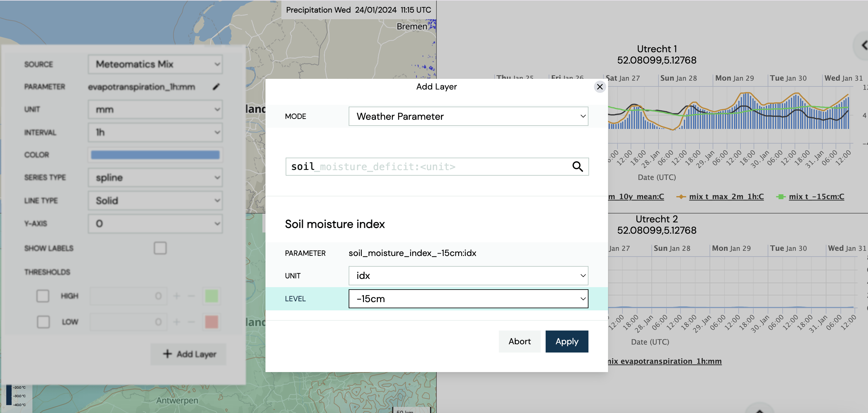
The next parameter that we add to this plot is the soil moisture index at a depth of 15 cm. Click on the ”Add Layer” button on the bottom right of the Layer Stack. Type ”soil” in the ”Search for weather parameters” box and click on ”Soil moisture index” (the second suggestion).
You can now specify the parameter properties (unit and level). In this example, we choose the unit ”idx” and a level of -15cm. Thus, the soil moisture index in a depth of 15cm is displayed after clicking the ”Apply” button.

If wished, you could now change the preferences of the soil moisture index by clicking on ”SPLINE soil_moisture_index_-15cm:idx” on the Layer Stack. In this example, we stick to the default setting.
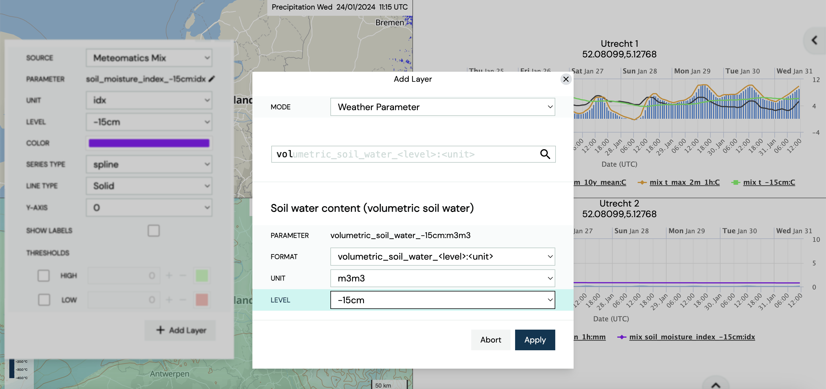
The final parameter that we add to this plot is the volumetric soil water. Click on the ”Add Layer” but- ton on the bottom right of the Layer Stack. Type ”vo” in the ”Search for weather parameters” box and click on ”Soil water content (volumetric soil water)” (the first suggestion).
Your final map should look like this:

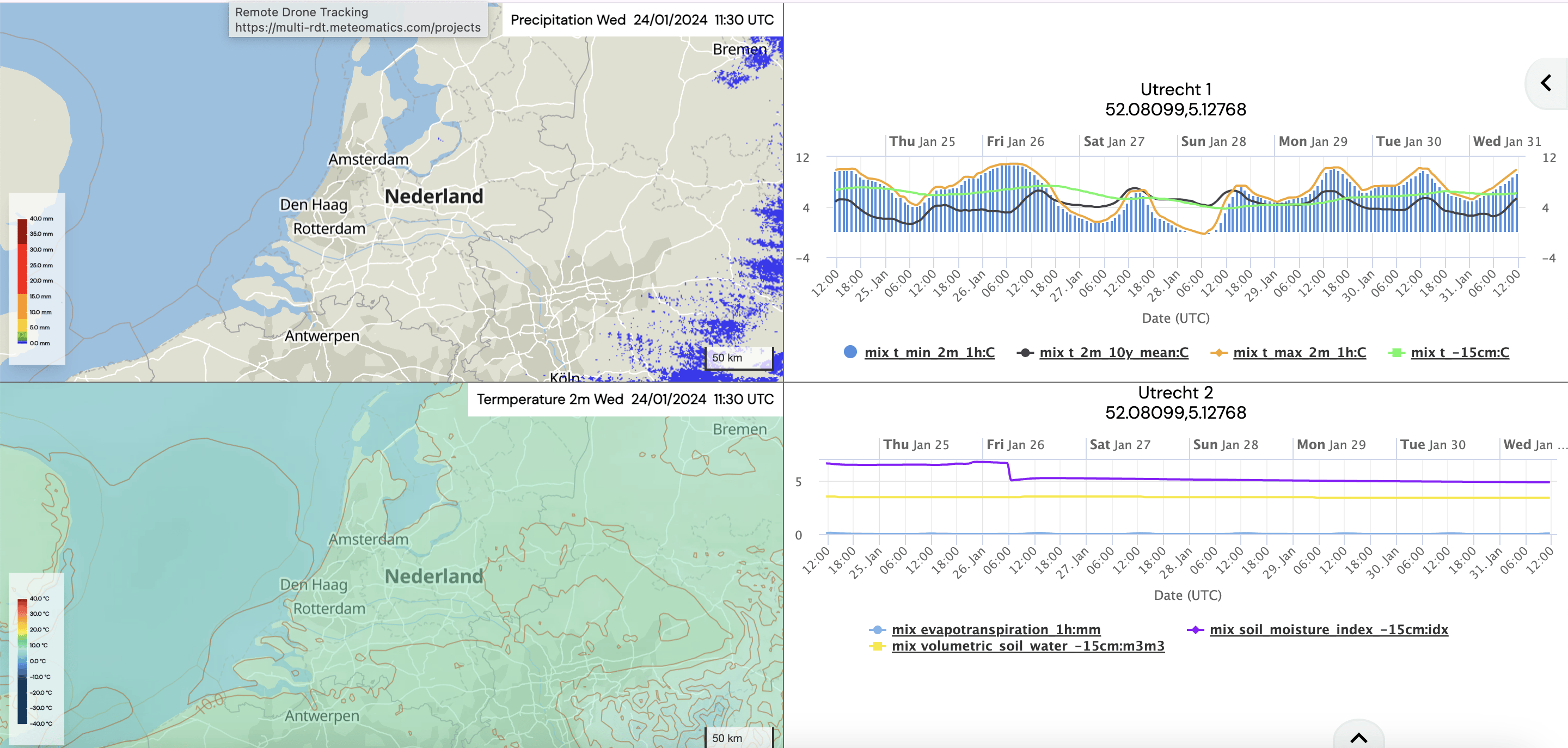
You can now switch to the animation mode, download the dashboard and share it with others or download an image.