Behind the Scenes: How to Program a Python Script for Regular Energy Weather Forecasting with Meteomatics Weather API

The quantity, quality and ready availability of Meteomatics weather data is ideally suited to customers in the energy sector, from modelling consumer demand to predicting renewable output and much more in between.

Customers from Hive Power, who value the long-term availability and accuracy of our weather data for their short-term power forecasting AI, to Heimdall Power, who are using our bespoke line-rating solutions to help in their goal of digitizing the power grid. Meteomatics serves more than 100 customers (BKW, EDF, ENEL, Axpo, Stadtwerke München, etc.) in the energy sector with highly accurate weather solutions and helps them to improve their daily operations every day.

To demonstrate just how easy it is to begin using Meteomatics data for your forecasting needs, in this article I’m going to show how I used the Python connector to create a script which produces an energy-relevant prognosis for the next few weeks. We now publish a short report on the output of this automated script every fortnight, which you can find at the news section of our homepage; alternatively, if you’re interested, you can contact me via [email protected] and I will send you a copy of the script, which provides a template for adapting a simple forecast to areas, timescales and variables of interest to you! Also, I’m happy to exchange ideas about possible improvements or new ideas.

What influences the energy market?

Of the great many factors which influence the cost of energy, the two most important can – somewhat broadly – be labelled ‘supply’ and ‘demand’. Weather influences both of these in a major way. On the demand side, consumer behavior changes dramatically as a result of what’s going on outside.

If it’s pouring with rain, people are more likely to sit indoors with their TV on, and, of course, the colder it gets, the more it’s going to take to keep everyone cozy in their homes and offices. On the supply side, as renewable sources provide a larger and larger share of global generation, predicting the total shortfall which must be compensated by dispatchable sources is essential in terms of keeping the grid balanced and the lights on.

Consequentially, two weather variables are of huge significance for the energy trading outlook in the short term. The first of these is temperature, which affects demand. In fact, more than just the absolute temperature itself, energy traders are often interested in temperature ‘anomaly’, that is, how does the temperature compare to the seasonal average. Folks expect things to get frosty around Christmas, but a sudden cold snap can mean that it feels much colder, and correspondingly drives heat demand much higher than is average for the time of year.

The second variable we share in our fortnightly briefing is wind speed, since this is the factor on which wind power generation depends. Another source of renewable energy is solar power, but we make no attempt to forecast this for two reasons: firstly that, in the absence of clouds, solar power generation depends almost exclusively on the number of daylight hours which, excepting a surprise eclipse, is extremely predictable; secondly that clouds, by contrast, are extremely difficult to predict, particularly on the timescales we include in our report.

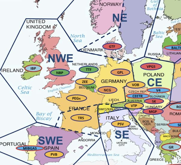
We provide time-series of this data for large geographical regions, giving an overview of the fluctuations energy traders should prepare for over the coming weeks. There’s a sweet spot to hit here: too many small areas makes the presented information difficult to interpret, but one big spatial average hardly applies over the whole of Europe. Our solution is to provide time-series which correspond to the regions covered by several large gas markets, and to supplement this information with an animated map of temperature and pressure¹, which gives an impression of changes from the averages represented in the time-series on a more local scale.

Our automated script produces these results for Europe. If you’re interested in how they look for your region, or want more granular information, go ahead and download a copy² and edit the configuration accordingly.

Given that the output of the script is a collection of plots, unit tests are somewhat difficult to implement. If it doesn’t work for your configuration, please get in touch at [email protected] and we’ll see what we can do to fix your issue and make the template more robust in the future. In the meantime, to help you debug and adapt the template, the code is written functionally, with only the major steps included in the __main__. Let’s have a look at what these steps are and how they were achieved:

Polygons and Geometries

The Meteomatics API allows users to retrieve time-series data for points and for all points in a regular grid. This is fantastic, but unfortunately geography is our enemy, and the vast majority of countries are not rectangular. We can get around this by using the API’s polygon query, which returns us a time-series of some aggregation (i.e. the mean) of all data within a non-square area. To use this though, we first have to define our polygons.

The API documentation will tell you that, to define a polygon, you have to provide a list of all the pairs of coordinates which constitute the boundary (each of which will be joined by a straight line). This sounds laborious, but the Python connector comes to our rescue! In my script, I demonstrate two easy ways of getting accurate polygons.

Both methods utilize the GeoPandas package. If you’re not familiar with this, it is a geographic extension of the incredibly popular Pandas package, which facilitates the manipulation of labelled data³. The major difference in GeoPandas is the addition, to each (Geo)DataFrame⁴, of a ‘geometry’ column, without which the GeoDataFrame is invalid. You can make any DataFrame into a GeoDataFrame by adding a geometry column, which must consist of Shapely objects. If all this seems daunting, don’t worry, it’s not hugely important⁵. We need GeoPandas primarily to leverage its built-in ‘naturalearth_lowres’ dataset – which provides polygons corresponding to every country in the world – and also to read in some other geometries which we’ll create. It is, however, worth noting that you will need to install GeoPandas to run my script, and that this can be a bit troublesome. I’d recommend creating a new environment in which to run the script, and installing GeoPandas before any other packages, since it can sometimes cause environments to break if dependencies are installed in a different order.

The first method is the easiest, but has some limitations. In my script, you’ll see that the argument ‘standard_countries’ is just a list of country names. These countries can be looked-up directly in naturalearth_lowres, so if you only ever need to use polygons representing entire nations you can just edit this list and skip to the next section!

The second method is slightly more arduous, but does have the handy consequence that you can define your own geometries, and it’s still much easier than listing the coordinates of all your polygon’s corners by hand. It utilizes GeoPandas ‘read_file’ method, which is essentially Pandas’ ‘read_csv’ adapted for GeoJSON data. In case you don’t have a GeoJSON handy for your intended polygon, let me show you how I made mine:

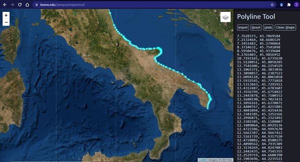
A multitude of tools exist for the drawing of polygons on maps. I used a tool provided by Keene State College, which instantly registers the coordinates of the points you right-click on the map in both a comma separated- and a JSON format. You can see an example of me doing so above. Simply keep clicking until you’re happy with your polygon, click ‘close up shape’ in the panel on the right, and copy-paste the JSON format data into a plaintext file.

Before you save it, add the highlighted text (immediately after the first open curly bracket):

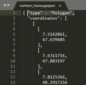
Now save your file, specifying its format as .geojson. Your computer may not register this as a recognized filetype, but that doesn’t matter – GeoPandas will read it no problem. Unless you’re competent at writing additional data to GeoJSON files, you’re going to have to name your manual geometries within the code. I do this using the ‘manual_geometries’ dictionary.

The second method is useful if you ever need to examine an area which is smaller than a country⁶, or if a country you’re interested in is sufficiently small that naturalearth_lowres doesn’t really do justice to it.

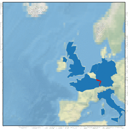
For large countries though, although you can make much more precise and pretty polygons with the second method, I was glad of the former, since mapping a coastline can take forever. Both methods are implemented in the get_geometries function, which takes an additional argument ‘show’ which allows you to visualize the resulting polygons on your map projection of choice to verify that they’ve been read in correctly.

In the picture below I’ve also used the overlay function of GeoPandas to draw the overlap between my manually drawn Northern France polygon and the coarse one of Germany automatically obtained from the built-in dataset.

Time-Series Data and Plots

Now that we have polygons corresponding to the geometries we’re interested in obtaining weather data for, producing time-series is as simple as requesting the data from the API and plotting the result.

In order to retrieve polygon data from the API, the coordinates of the polygon must be formatted in a specific way: a list of pairs of coordinates per polygon. This is handled by my make_tuple_lists function. In the case that a region of interest consists of a single polygon the function wraps the list of coordinates inside another list since, in general, the list may contain multiple polygons – this is the case for Italy, which includes the islands of Sicily and Sardinia. A polygon query can only return some aggregation of the data within the polygon as a time-series, meaning that – even for Italy – only a single time-series is ever returned (if you wanted to avoid this, you’d have to parse the separate islands as separate manual geometries). You may notice that the polygon request is made separately to the call to the plotting function within __main__. The reason for this is that it is desirable to consider the data from all polygons in order to set global maxima and minima for y-axes on the plots for easy comparison. The resulting time-series plots for two of the regions I consider in my script are shown below.

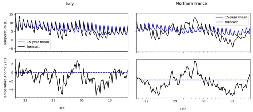
The upper panels of these plots show the forecast for the next 28 days at the time of writing alongside the climatological background on the same scale. The lower panels show an alternative view of exactly the same information: by subtracting the background from both lines from the upper panel we get the difference between the data and the historical average. This is clearly zero for the background itself, and a dotted line is included to highlight the departure of the forecast from the climatology. Period where this difference is greater than zero may lead to higher-than-average demand, and vice versa for periods where the difference is less than zero.

A quick comment on the climatology: different disciplines may have different standards for the length of time required to build an accurate average picture. An accurate mean would ideally include as much historical data as possible, but there are two limitations to this: accurate records of weather data may not extend much further back than 1980 for many regions worldwide; and the effects of climate change, as well as socio-economic data one might want to compare against⁷, might mean that more recent data is more relevant to the questions being asked. The standard length of background period in climate science is 30 years; in power forecasting it is more usually 15 (according to our industry experts). The script can be configured for either of these, or any other length of time. In order to save on runtime (which can be lengthy if a long background is sought), the climatology is calculated as needed and saved to file, from which it can be read more quickly in future. Users should be aware that an up-to-date climatology is important for accurate anomaly calculation, and the climatology should be re-built periodically – preferably once per year.

Map Data and Animation

These time-series plots are useful for clearly and quantitatively showing how important weather factors are due to differ from the long-term average in our forecasts, but have the disadvantage that they reduce large geographical areas to single data points for each time step. In order to get some idea of the variation we might see over our polygons, as well as the weather systems which are responsible for the patterns we see in the time-series, it is of interest to view the weather situation in pictures, a series of which can be animated to see the development of the situation over time.

My script makes animations from pictures of temperature – represented by a color scale – and pressure – represented by contours (also called isobars). In contrast to the time-series plots, it is not straightforward to edit- or add to the variables shown, since in general different representations will be optimal for different data (for instance, wind might be best represented by arrows or barbs; showing precipitation might require that either the contours or the color scale is replaced by rainfall amount). However, a great many things can be inferred from a synoptic-scale pressure chart.

The script makes animations by retrieving gridded time-series from the Meteomatics API, which can be converted to an Xarray Dataset⁸ for convenience. Depending on the map projection chosen, the latitudes and longitudes associated with the retrieved data will need to be converted so that the result can be plotted on a map. I then plot each time-step separately before calling Pillow to convert the images into a GIF. The individual images are preserved though, so you can step through them at a more leisurely pace if you like.

Possible Improvements

Our fortnightly update is by design a top-level summary of the weather situation in Europe. I hope the template I’ve provided is helpful, but depending on your exact needs, many things may need to be changed. I’ll end this article with a short discussion of some of the most important factors to consider.

Energy demand is influenced to a greater- or lesser extent by a great many factors. Even heating demand, which is indicated by the temperature time-series we produce, is in reality much more complicated. Our time-series is an average of all the points within a given polygon, which may not be representative of the real distribution of population. For instance, in the UK, roughly a 10^th of the population live in the greater London area; very few, relatively, live in the Scottish highlands. Hence an average temperature for the whole country – which is likely affected considerably by the expansive and generally much cooler northern regions – may not correlate perfectly with the temperature in London and other urban centers, from which much of the share of demand may originate. A crass solution to this problem would be to further subdivide the UK into smaller regions containing these urban areas; a more mathematically rigorous technique might involve obtaining spatial data (e.g. from a grid time-series request) and weighting by population density.

In addition to the uneven distribution of population, factors such as quality of insulation, local affluence/fuel poverty and day of the week will affect the demand response to temperature. It is also true that even temperature anomaly is not necessarily the best indicator of how people will respond to temperature. For instance, National Grid have concluded that people are more likely to turn their heating up if today feels a lot colder than yesterday, and attempt to capture this in their ‘effective temperature’ calculation.

Heating is also not the only consideration for demand modelling. Although less prevalent in Northern Europe, in many parts of the world warm temperatures also imply a significant change in energy requirements due to air conditioning. The temperature – as well as many other weather factors – may also affect many auxiliary energy costs, depending on the work- and leisure activities of the local population.

Similarly to temperature on the demand side, energy generation by wind power sources will generally be modelled much better by considering the forecast for specific regions which contain wind farms. If you operate a wind farm, our code can easily be adapted for your purposes with a few specific custom geometries. You might also be interested in changing the weather variable used in the wind forecast. That included in our report is the 90m wind speed, since this is the average hub height of an onshore wind turbine. For offshore farms, a different height may be preferred. For many standard weather parameters – of which wind is one – the Meteomatics API allows users to retrieve data from a continuous range of interpolated heights, so you can get accurate data whatever your hub height!

Although broadly speaking a higher wind speed implies a higher power output from turbines, this relationship is not linear. Instead, the results of a wind query will need to be put through a ‘power curve’ to obtain the output, essentially to model the fact that very low wind speeds will not turn a turbine efficiently; that peak efficiency is reached at about 15ms^-1; and that the turbine has to be shut down at dangerously high speeds, hence producing nothing.

Additionally, operators of wind farms will be well aware that other fluid effects, such as the blockage and wake effects, are significant when considering clusters of turbines in close proximity. Luckily, Meteomatics downscales all API data to a 60m horizontal resolution, meaning that we’re still an ideal choice of data source for high-resolution modelling of such effects.

These suggestions only cover the variables which we include in our update. Of course, if you were to use this template to examine other data – whether for energy forecasting or for any other purpose – a different set of assumptions and corrections will be required. The important thing to remember is that, whatever your ambition, Meteomatics provides the weather data you need to make it a reality, and that our team are more than happy to help with bespoke solutions to your problems. Get in touch today to find out how you can start leveraging the capabilities of the world’s most powerful weather API!