Watershed Delineation With Pysheds

The watershed of a river is the boundary within which a drop of water would drain into the ocean at the same estuary¹. More generally, a watershed can be defined by a ‘pour point’ (the estuary in the case of an entire river) further upstream, meaning that if you query rainfall data within the watershed, you can predict things like the volume/flow rate of water at the pour point.

Decision makers in multiple arenas might find application for the delineation of a watershed. For instance, in town planning, it may be useful to find the catchment area of a river to aid with flood extent prediction, whilst in power forecasting the operators of hydro plants can use the watershed to estimate energy delivery. In this post I show how you can determine catchment areas and flow rates for any body of water using Meteomatics’ highly resolved elevation data, available through our API.

PySheds

The pysheds library contains functions/methods which allow you to read .tiff files and delineate watersheds. You might not have access to a .tiff file, but as a Meteomatics subscriber you can use our API to obtain a digital elevation model (DEM) and find the boundary of a watershed yourself. I’ll show you how to do this, and how to retrieve rainfall data corresponding to the watershed.

Here you can see the structure of my API request for elevation data. By default the data here is obtained from the NASA SRTM/ASTER model, which has a ground resolution of approximately 90m. This is the same model we use to downscale coarse resolution weather model output so that data accessed through the Meteomatics API is updated according to the local geography of a request. `bounds` is a dictionary which contains the edge coordinates of the region I’m interested in, and `res` is a variable which determines the resolution of the data to be acquired.

I’d recommend as high a resolution as possible, since the more information about the local slope you’re able to extract from the API, the better your watershed picture will look. That said:

a) Some rivers will have huge catchment areas which, at high resolution, may exceed the maximum number of data points in a single API request²

b) A resolution of 0.001 degrees roughly corresponds to 100m, so requesting data at a higher resolution than this is unnecessary, since it is smaller than our downscaled data

The datetime object I pass as the first argument to the request is arbitrary, since we don’t expect elevation to change very much over time.

Next I replace all locations where elevation is zero to NaN, and turn the data I retrieved from the API into a netCDF (an industry standard format, necessary for the next step). Since 0m elevation could equivalently be stated as ‘at sea level’, this essentially removes the ocean from our data. This is important, because otherwise water would be allowed to flow forever over this perfectly flat surface, which is clearly unphysical.

elev[elev <= 0.0] = np.nan
da = elev.T.unstack().to_xarray()
nc = da.to_dataset(name='elevation')

Now that we’ve got a netCDF of elevation, we need to install the rioxarray package. This package works with xarray (a package for manipulating netCDF data which you should also install) to facilitate the writing of TIFF files. After installing these packages using the

`pip install -c conda-forge <package>`

command, you can implement the following:

nc.rio.set_spatial_dims( 'lon', 'lat', inplace=True)
nc.rio.set_crs("epsg:4326", inplace=True)
nc.rio.to_raster('elevation.tif') 
grid = pysheds.grid.Grid.from_raster('elevation.tif')
dem = grid.read_raster('elevation.tif')

This gets you a digital elevation model in the format desired by pysheds. Let’s take a look at our DEM.

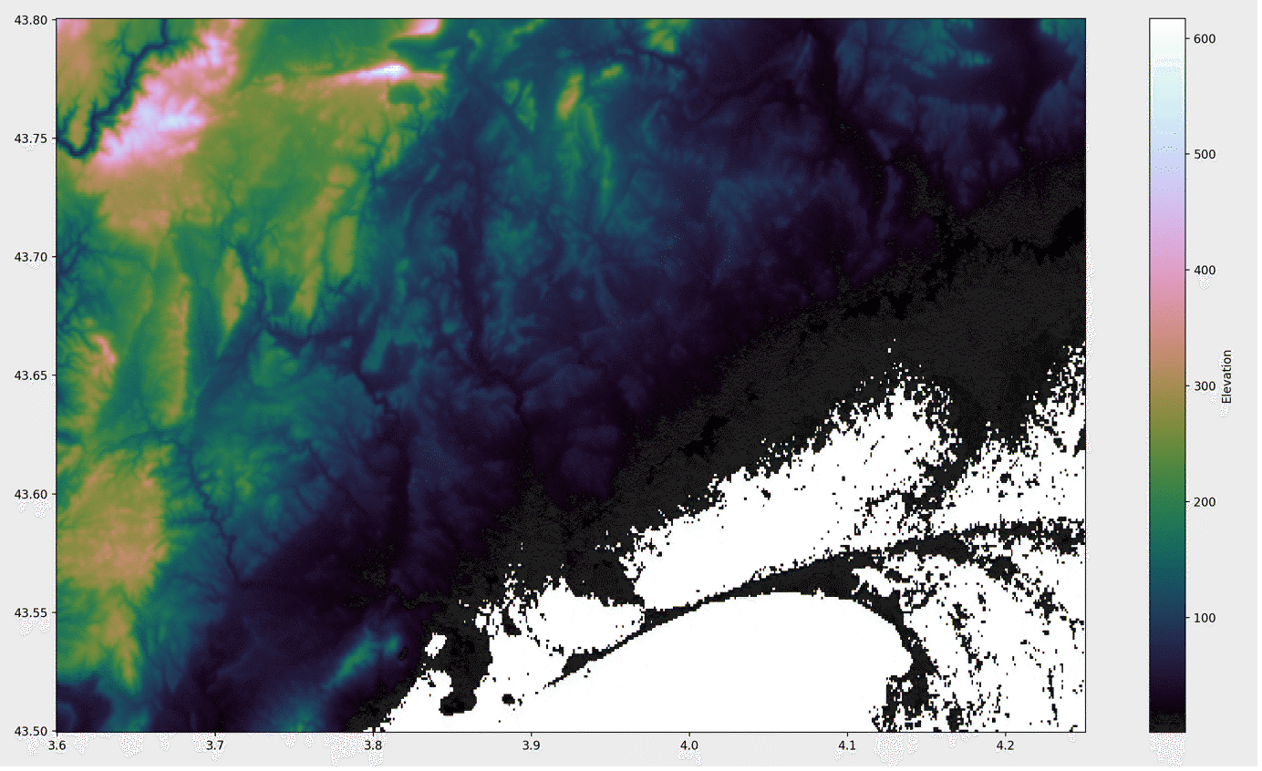
We’re now almost ready to delineate a watershed. Before we do, however, we need to take care of any small artefacts which may exist in our DEM. pysheds refers to these artefacts as pits and depressions, which are localities where the surrounding area is all higher than the artefact (hence water can pool there), and flats, which are areas of constant elevation. We already removed the most challenging (and unrealistic) flat – the sea. We can remove the others, as well as the pits and depressions, very easily using the following methods on the DEM object:

dem = grid.fill_pits(dem)
dem = grid.fill_depressions(dem)
dem = grid.resolve_flats(dem)

We should now check that we have successfully removed all the artefacts as described above

assert not grid.detect_pits(dem).any()
assert not grid.detect_depressions(dem).any()
assert not grid.detect_flats(dem).any()

If you get any assertion errors here, something has gone wrong. I found that all of these disappeared after I had correctly masked the ocean from my data, but if the errors persist you’ll have to examine the DEM in detail to see where things are going wrong. Fortunately, failing these assertions doesn’t prevent us from computing the next steps, and the results of these can be useful when trying to analyze where the error may be.

We can now calculate the flow direction and accumulation of the DEM as follows:

fdir = grid.flowdir(dem)
acc = grid.accumulation(fdir)

Flow direction is a number between 0 and 360 representing the direction of flow of the watershed at every given point. Accumulation quantifies the cells in the DEM which are upstream of the cell in question. This is a useful property to know for several reasons, as we will see. The code below generates a map of the rivers in our DEM, which I show in figure 2.

f = plt.figure()
ax = f.add_subplot(111)
f.patch.set_alpha(0)
im = ax.pcolormesh(
 nc.lon, nc.lat, masked_acc, zorder=2, 
 cmap='cubehelix', norm=colors.LogNorm(1, acc.max())
)
plt.colorbar(im, ax=ax, label='Upstream Cells')
plt.title(
 f'Flow Accumulation in catchment\n of pour point at {x_snap},{y_snap}', 
 size=14
)
plt.tight_layout()
plt.show()

The color scale of the picture is the variable acc. You can see that cells located on the slopes of valleys have very few upstream cells – hardly anything flows towards them – whilst the accumulation of rivers increases as they flow towards the coast – every cell downstream is fed by at least one upstream cell. This means that we can use accumulation as a proxy for how far downstream we are, and can also set a reasonable value of accumulation to distinguish flowing rivers from hillside.

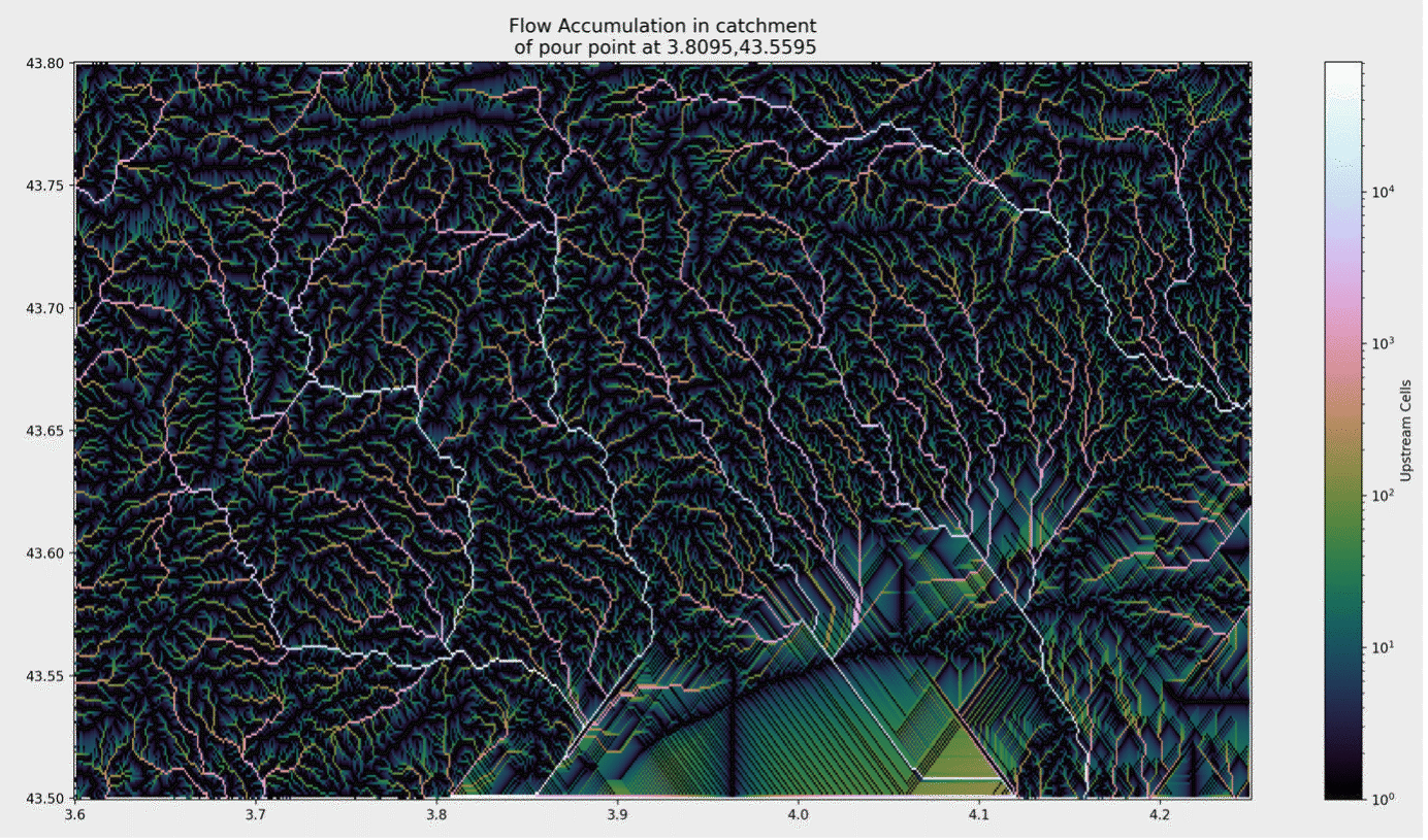
You can see that, as we discussed earlier, our rivers don’t really know how to behave when they hit the ocean. This is unimportant, since flow isn’t quantified here, and we can just mask those parts of the domain.

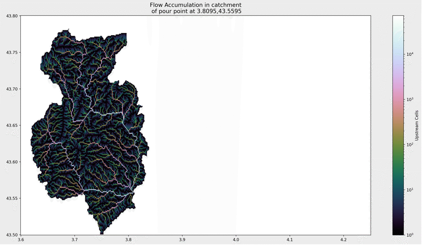
Now it straightforward to delineate a catchment for a river. We simply need the coordinates of the ‘pour point’. This can be the point at which the river flows into the sea, or a point further upstream that you’re interested in. For my example in Montpellier, I’m interested in the location that the Lez and the Mosson meet. This is at about 3.81, 43.56. We type the coordinate into our code, but also make sure we snap to a nearby point with enough accumulation: it would be embarrassing if the result of the next step showed us a tiny area because we’d accidentally picked some nearby hillside instead of a point in the river…

# Specify pour point
x, y = 3.8095, 43.5588
 
# Snap pour point to high accumulation cell
x_snap, y_snap = grid.snap_to_mask(acc > 10000, (x, y)) 
catch = grid.catchment(x=x_snap, y=y_snap, fdir=fdir, xytype='coordinate')
masked_acc = np.ma.masked_array(acc, catch==False)

We then find the catchment area using the catch method of the grid object. This is a Boolean field describing whether or not a cell is in the catchment. I mask my accumulation according to the catchment, and show the result below

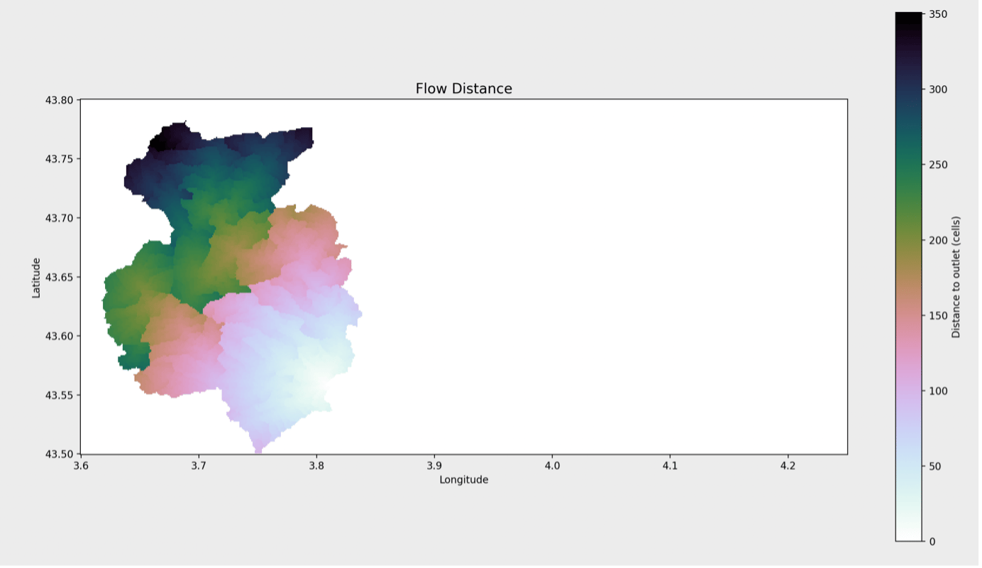
From this it’s easy enough to categorize the area according to the distance to the pour point

dist = grid.distance_to_outlet(
 x=x_snap, y=y_snap, fdir=fdir, xytype='coordinate'
)

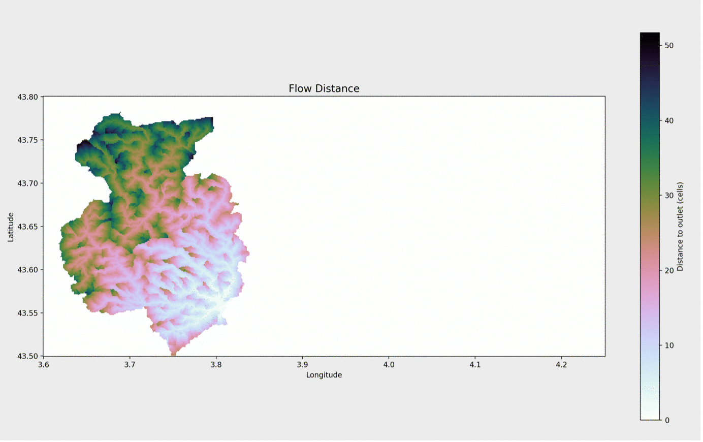
and it doesn’t take much more to categorize the region according to how much time it would take for water in each cell to get to the pour point. All we have to do is implement a simple assumption – say, that water in a river (i.e. a cell with a lot of upstream cells) flows about 10x as fast as water on a slope

weights = acc.copy()

weights[acc >= 100] = 0.1

weights[(0 < acc) & (acc < 100)] = 1.

The pysheds package is potentially immensely useful for any application associated with river levels and flow. Some of these are shown or described in this article, but there are many more ready to be exploited by users with access to such a high-quality DEM as is provided to Meteomatics’ API subscribers.

You can find information about our additional geographical data here. As usual, if you have any questions about the use of our data or about the techniques explored in this article, feel free to contact me using the form below!