Flood Extent Calculation with Pysheds

A few weeks ago, I published a blog post showing how we can use Meteomatics’ elevation data as a DEM to delineate watersheds. In this article I’m going to apply this to the use-case of modelling flood risk zones around riverbanks.

Flood Waters

Let’s say you’re planning the development of some housing or infrastructure, and you want to know how exposed to flood risk your projects are at certain locations. Perhaps you know that during a small flood event a local river bursts its banks by X meters.

Using the methods outlined in our previous post, we can map the catchment area of the river under consideration. The pysheds package we used to do this also facilitates the calculation of the ‘height above nearest drainage’ (HAND). By this we mean how many meters of elevation separate each cell in the DEM from the nearest cell considered to be a ‘drainage’ cell, i.e. a cell in a waterway which will transport water arriving at it rapidly downstream. These drainage cells are identifiable since they will have a large number of upstream cells flowing into them.

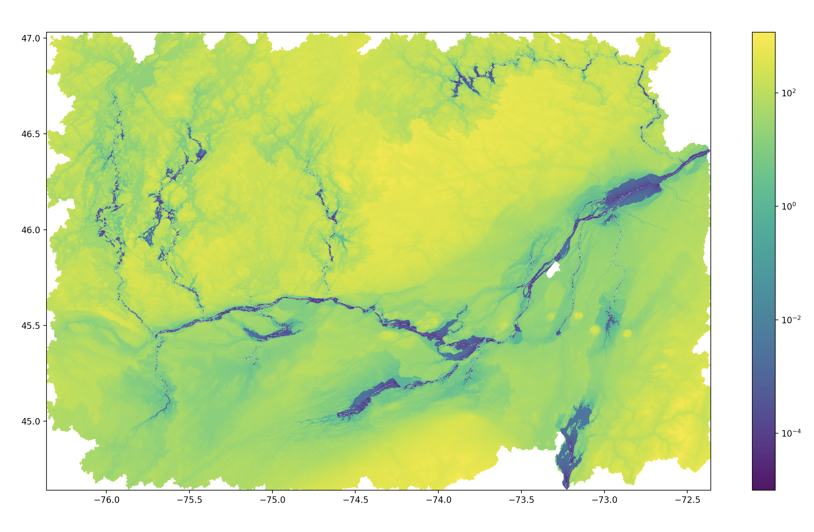
In Figure 1 I show the HAND of a stretch of the Ottawa river in northeast Canada. The scale is logarithmic, and the river can be seen as the blue line through the centre (all water bodies, including the tributaries to the north and south, appear blue, as they themselves represent the nearest drainage, hence are not above it). I chose the definition of a water channel as the value of accumulation¹ at approximately (77.7W, 45.4N) because it is a convenient junction of the river at a location significantly upstream of Ottawa city. Plenty of smaller tributaries in the geographical region shown are therefore not visible, as they feature fewer upstream cells² than the point I chose.

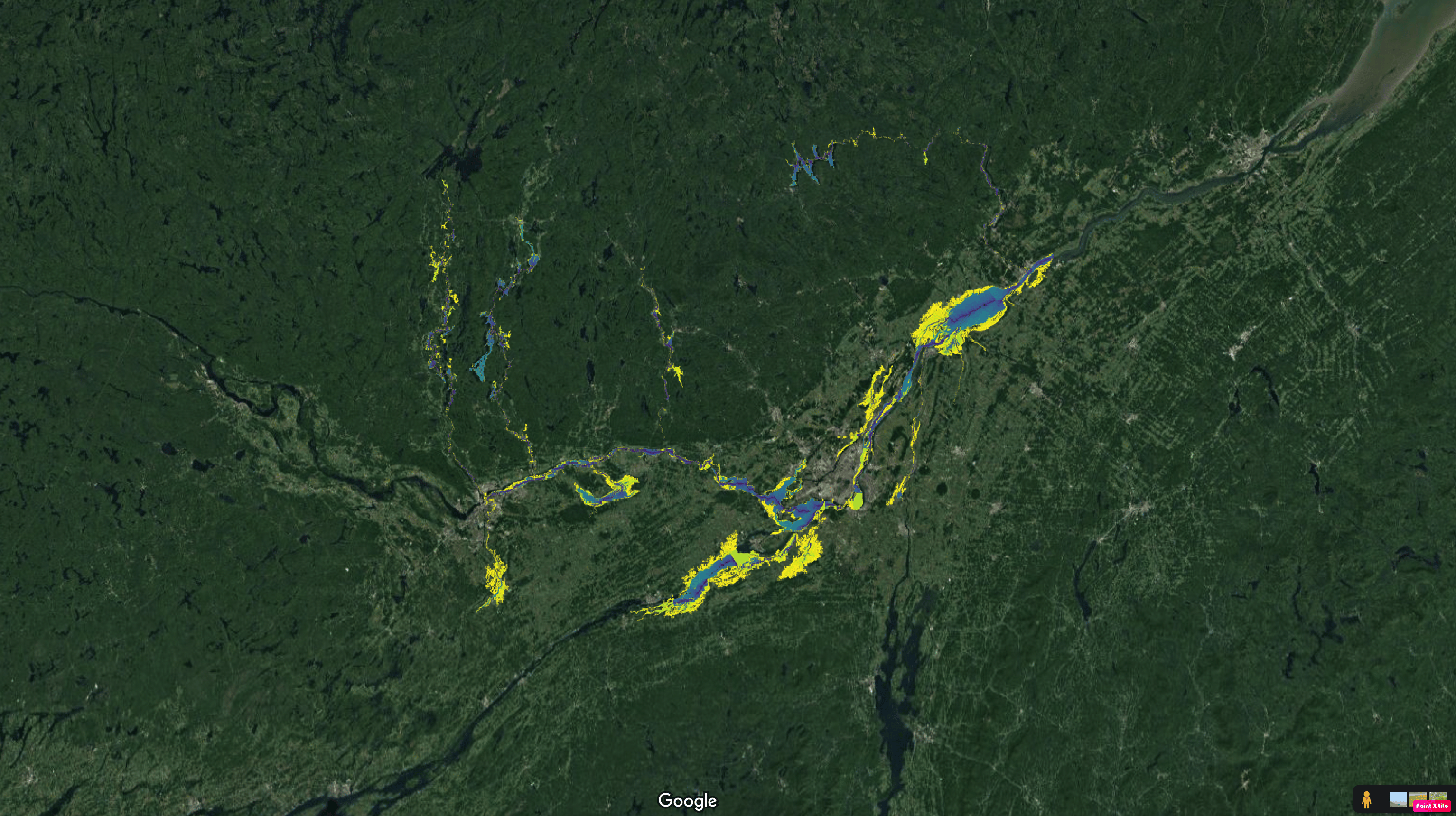
I was then able to mask all the cells from Figure 1 where the HAND was less than 5m, and I show this in Figure 2. 5m would represent a historically unprecedented flood for the Ottawa region, but illustrates the point that by overlaying the HAND on a satellite image we can show the spatial extent of floods and reveal the areas of existing or planned development that are at risk from events of this magnitude.

Return Periods

If we want to obtain more realistic results from our flood modelling, we need to consider what is reasonable, given historical river level data.

One way of achieving this is to consider the concept of ‘return periods’. If you’ve ever seen reporting about floods or other climate events in the media, chances are you’ll have encountered these. Whenever a reporter describes a disaster as a ‘one in a hundred year event’, they’re talking in terms of return periods. The language used in such reporting is a bit misleading: what this actually means is that, on average, we’d expect events of this magnitude to occur 100 years apart³ This doesn’t preclude two 100-year events from happening two years apart, nor does it guarantee that a 100-year event will happen next year if none have occurred in the previous 99. A better way to think of the return period is as an inverse of the probability: if in any given year the chances of an event happening are 1/100, the event has a return period of 100 years.

By studying an historical record of river heights, we can determine the floodwater levels associated with events with various return periods. The methods which I'll describe in the next section are slightly different but have advantages and disadvantages when it comes to allowing us to determine return periods.

For both methods, we first find the approximate return period of the flood values we have on record. To do so, we resample our time-series data. If your river height time-series is at sub-daily resolution, you’ll need to first resample it to extract the maximum daily height. Once you have this, you can resample again to get the maximum daily height within a year. You’ll now have a time-series with as many data points as there are years in your dataset, and each data point will represent the largest flood event in the given year.

Next you’ll need to use Weibull’s approximation to determine the return period of each flood. In the formula

P = (m+1)/n

m is the rank of the observed annual maxima when arranged in descending order, n is the total number of years on record, and P is the probability of exceedance. The lowest annual maximal river height you have has an almost 100% chance of being exceeded every year; the highest was only seen in one year in your record, so the chances of exceeding it are correspondingly smaller.

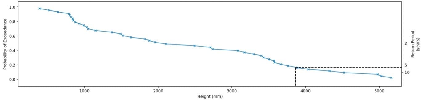
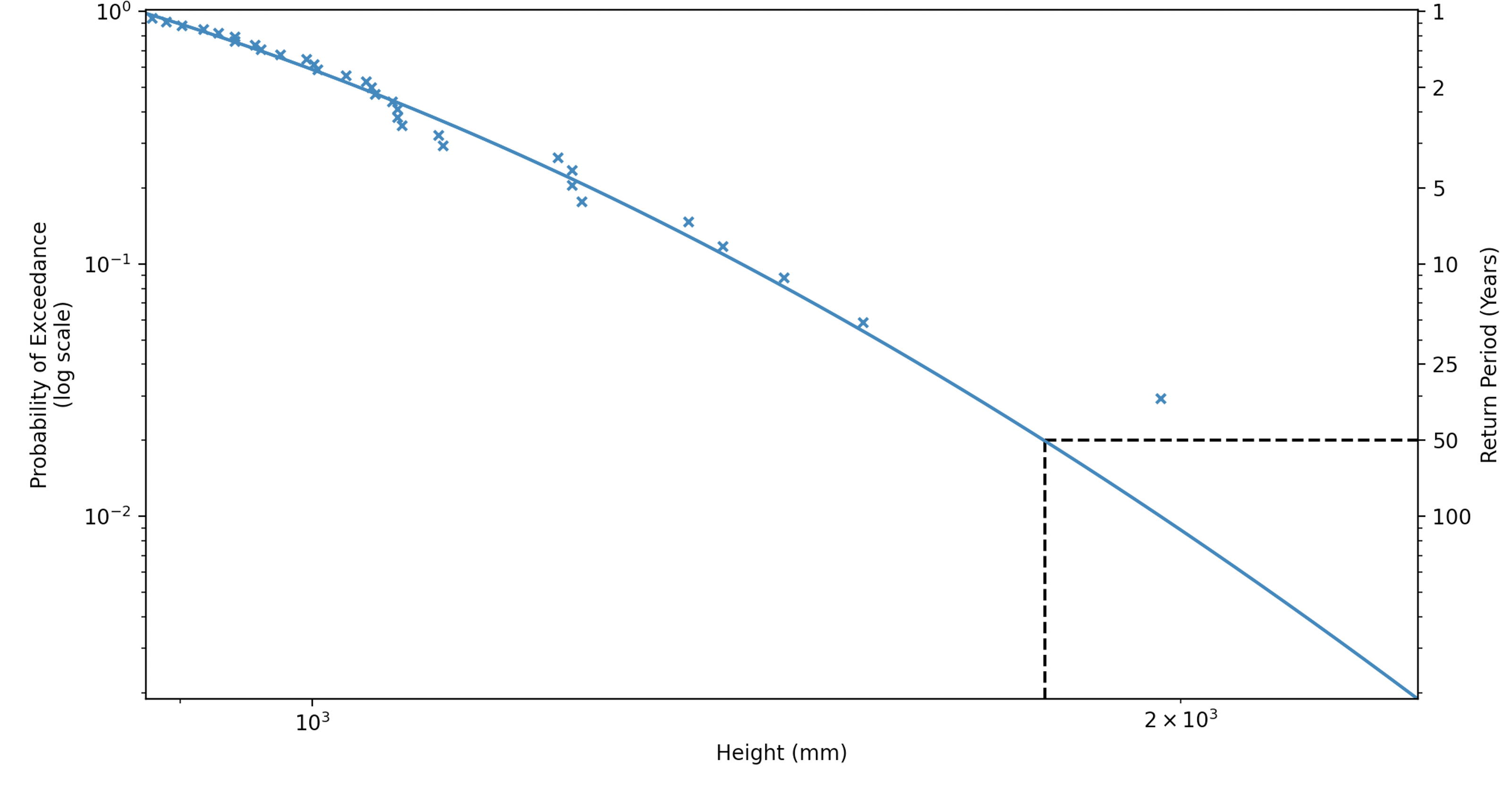
Method 1 involves simply linearly interpolating between these exceedance probabilities to obtain the heights corresponding to the return periods you want to know. Recall that these return periods are the inverse of the exceedance probabilities, so if you want to find the 25-year return period water level, you’ll need to find the value which is exceeded with a probability of 1/25 = 0.04. Figure 3 shows a plot of the actual annual maxima and their corresponding probabilities, and illustrates how you can read off a river level value for a probability (and hence return period) of your choice.

Method 1 facilitates the precise calculation of return periods within the range of available data. If, however, you wanted to estimate the magnitude of a 50-year event, but only have a record covering 40 years, you need to be able to extend your record somehow.

Method 2 achieves this by fitting a model to the data. The chosen model should be a probability distribution, since the data to be modelled (the y-axis in figure 3) is a probability. There are, however, many probability distributions, of which not all will be appropriate. Since the kinds of events we want to predict are very rare, belonging to the long ‘tail’ to the right of the distribution, we require an extreme value distribution. There are several of these, each appropriate for different modelling assumptions, but I chose a log Pearson type III distribution. Now, since we can extend the modelled distribution over any range of flood height values, we can obtain any return period height we like, including those outside the range of our record.

We can see that the model used in method 2 introduces some discrepancies. MORE ON THIS. It’s not so easy to say that these are ‘errors’, since the values obtained using method 1 are themselves estimates, but clearly there are differences. We expect longer records of water levels to produce more reliable results with both methods, but these are not always available. You can of course play around with various different probability models for method 2, but it’s often good to mirror some industry standard for simplicity of comparison.

There are two advantages to having calculated return periods using the method(s) described above:

1. The flood extents we can visualize in our DEM now have a basis in physical reality – we can map events which may actually happen, with real estimates of their likelihoods.
2. If we include return period estimates from several stations, we can interpolate the floodwater heights between the measurement locations, obtaining an even better estimate of flood impacts.