Creating a Julia Connector for Meteomatics' Weather API

Here at Meteomatics it’s our mission to make our API as easy to use and integrate into your workflow as possible. One of the ways we achieve this is by providing connectors to our API for all kinds of software including standard data analysis programs such as Excel and Tableau, geographic information system software such as ArcGIS and QGIS, and of course all the most popular programming languages.

In contrast to the aforementioned categories of software, which have limitations on the operations that a user can perform built into the program, all computer languages are theoretically capable of doing exactly the same things. A relevant question then is “why bother with a connector for every language?”. The answer – that our customers use a variety of different languages – is not overly satisfying: why does such a variety exist at all?

The reasons that a plethora of different programming languages are available today can essentially be boiled down to two principles: some languages aim to make it simpler and more intuitive for humans to read and write code, hence accelerating the rate at which new code can be developed and understood; meanwhile, other languages focus on creating more precise and therefore efficient instructions for the computer which implements the code, reducing runtime and memory requirements.

These two design principles often trade off against one another – the easier it is for a human to read and write code, typically, the slower and more memory-intensive it will be to run, and vice versa. Still, the improvements in computer hardware mean that, even in a dynamically typed, interpreted (1) language like Python, programs run much faster on modern machines than low level languages ever did on punched cards.

For decades now, computer languages and their adherents have been fighting it out on the battlefield of efficiency vs readability. In recent years, a new combatant has entered the fray, promising to mediate between the warring factions and lead us forward to a future where computer programming can be easy to read and write, collaborative, versatile and efficient. This language is named Julia, and at Meteomatics we’ve just released the first version of a Julia connector. Those who already know what Julia offers and just want to get their teeth stuck into our new connector can head straight to GitHub. If, on the other hand, your interest has been piqued, and you want to know more about this exciting new programming language and our implementation, read on!

What makes Julia so great?

Although I learned to code in C (2), in my years of being a Python programmer I’d forgotten about a few intricacies that define how different languages work internally. Two of these are relevant for discussing Julia.

Typing and Compiling

The key to why, as I mentioned earlier, computer languages are all fundamentally capable of the same things is that all computer operations are performed by sending binary instructions to a CPU, which is capable of turning a string of 1’s and 0’s into complex operations (3). The difference between a compiled and interpreted code is in how the ‘source code’ (written by the programmer) is translated into ‘machine code’ (understood by the CPU). Compilation translates the source code all at once before running the program, whereas an interpreter, translates statements as they are encountered. Compiled code is faster because the translation is done ahead of runtime. However, in order to successfully compile, the whole program must make sense, including the bits which aren’t encountered. Interpreted code, by contrast, is slower to run but easier to debug, since the program can always proceed as far as the first failed statement.

Julia belongs to a group of modern computer languages which implement ‘just-in-time’ (JIT) compiling, which attempts to split the difference between these two methods. It is therefore easier to debug than compiled languages but, once complete, runs just as fast as they do.

Julia is also ‘dynamically typed’, meaning that variables are not constrained to have a single type, but can instead mutate during the flow of code. ‘Statically typed’ languages, where variable types need to be declared when a variable is initialized, catch a large class of errors early (often at compile- rather than runtime), and this makes it slightly easier to collaborate on code, since the format of variables returned from functions is always explicit. The advantage of dynamic typing is essentially that code is more forgiving to the programmer, although unexpected errors can sometimes appear down the line and be difficult to trace back to a source.

Taken together, the dynamic typing and JIT compiling of Julia are designed to make the language relatively easy to learn and intuitive to write. These principles should, however, be familiar to anyone who has ever written Python code. Additionally, Python has the benefit of many years of development, and consequently a huge number of libraries for doing all sorts of tasks, some of which are yet to be developed for Julia. So, I hear you ask, why bother?

Multiple Dispatch

The definitive feature of Julia which sets it apart from most other languages is its ‘multiple dispatch paradigm’. This feature, which is relatively easy to describe, ends up having a number of knock-on effects for Julia which are highly desirable.

Multiple dispatch essentially means that functions are defined multiple times in Julia depending on the types of the variables they take. A toy example gives the general idea (4). First, we create two new data types – Cat and Dog – both of which are Pets.

An abstract type is different to a concrete type (struct) in that instances of it cannot be created. It is useful for placing types in a type tree, which in turn is useful for defining fallback behavior, as we’ll see. To briefly summarize the rest of the syntax in the above: `<:` means that the left type is an immediate subtype of the right type; `::` means that the variable has this type i.e. the ‘name’ field of our pets must be a String; Julia uses `end` to end blocks of code, rather than tabbing as in Python (although there is no rule against tabbing and I include it to aid readability); and strings in Julia are enclosed by `”`, and the `$` symbol is used for string interpolation.

The function defined above will print a string stating what occurs when `a` encounters `b`, provided `a` and `b` are both Pets. The missing piece of the puzzle is the `meets` function, which we will now define.

This function has been defined four times, but we haven’t overwritten any of the previous definitions. Each definition is called a ‘method’ of the function, and the method utilized at runtime depends on the types of the variables passed. Let’s create some Pets and see how our code behaves:

So we can see how the data types of our variables affect the execution of a function which has the same name each time it is called. We’ve already used the supertype Pet to make sure a type error is raised if the types passed to `encounter` are not Pets i.e.

but we can also use it to implement a more generic method for `meets`:

This toy example demonstrates succinctly the implementation of multiple dispatch in Julia, but why is it useful? There are three main consequences of this paradigm which are beginning to attract converts from other languages.

Code reuse

The fact that the various methods of a Julia function are all named identically, combined with the language’s dynamic approach to typing, means that, when writing code, we don’t have to think too hard about the types of our variables. In Python, achieving the same results as our toy example above would require either that we defined the `meets` function as a method on Cat/Dog objects (5), or require several functions with non-identical names (e.g. `cat_meets_dog()`; `dog_meets_dog()`) be defined.

The problem with the latter approach is clear: the user has to remember the function required for each set of input types. The former limitations of the former approach are that the methods are bound to the object: the method cannot be used unless an instance of the object exists, can only be used on the given object, and cannot easily be extended to cover new behavior of new/updated objects. Both of these problems scale with the number of input variables to the function – in our toy example there are only two variables for each method, but this needn’t be the case: there is no limit to the number of arguments Julia methods can be ‘dispatched’ on, and different methods of the same function needn’t necessarily even take the same number of arguments.

As abstract as this sounds, there is a practical benefit to building code with unbound generic functions: it is incredibly easy to re-use code! Define a function – or extend an existing one – to handle a new data type, and all you need to do in order to use it in future is import it. Because Julia is a relatively new language, some operations you might be used to in your previous language of choice may not have been implemented, but you only need to implement them yourself once (6).

Package compatibility

A perhaps-not-obvious result of this ease of code re-use is that well-defined methods/data types propagate through other people’s code too! Since the names of the functions called never change, packages interoperate seamlessly without ever being specifically designed to do so. A frequently cited example of this is the compatibility of the DifferentialEquations and Measurements packages. The former of these provides a toolkit for solving differential equations of all stripes; the latter allows users to add uncertainty to their data. The magic of Julia is that, by plugging data types from Measurements into solver functions from DifferentialEquations, we can obtain a solution which correctly propagates error!

Efficiency

Perhaps the most cited advantage of Julia over Python is its relative efficiency. Julia can run up to 10x faster than Python, which may not be super important for simple code that takes seconds to run, but can scale up quickly when considering, for instance, complex numerical weather prediction code which can easily take days. Part of this efficiency comes from the JIT compiling of Julia, but another factor is the leveraging of multiple dispatch for efficiency.

A good example of this for those familiar with linear algebra is that of the ‘one-hot vector’. A one-hot vector is a vector which is uniformly 0 except for one index, which contains a 1. Without going into the specifics of matrix multiplication, this means that an inner product of the one-hot vector V with the matrix where M is

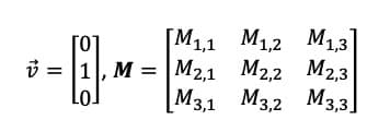
is

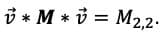
This result can immediately be obtained from knowledge of the index where

is non-zero, and is much faster than following the complicated process of multiplying matrices through all its tedious steps.

In Julia, this can easily be achieved by creating a struct for the one-hot vector (7) and extending inner product methods for this new data type. The mathematically minded ought to be able to think of numerous examples of special case shortcuts which they’ve encountered in their studies which could be coded in such a way; the field of linear algebra is rife with them, making Julia an extremely powerful language for efficiently processing matrices, with implications for all the fields – such as the vogueish machine learning – which require this. The example above might imply that, in order to use Julia at optimum efficiency, users would have to recognize opportunities to implement these shortcuts, but in fact even low-level arithmetic operations have different built-in methods to dispatch on basic types such as Integer vs Float, and many other speed-up implementations are included in popular packages.

Our Connector

The most conspicuous use of the multiple dispatch system in our Julia connector is in the case-switching implied by various methods of the query functions. Rather than throw errors when a user provides a date/time string to a function, for instance, the ParserFunctions module defines several methods for handling different inputs. This design lends itself more to the increased ease of use/ compatibility than increased efficiency of multiple dispatch, but is nevertheless useful.

One must be careful about when and where to use multiple dispatch. In our connector, a single `query` function could feasibly have been written which returned different results depending on the input parameters – a time-series if date/time ranges and intervals were provided; a grid if a single date/time was given for bounding latitudes and longitudes. However my decision, and I think a good guiding principle to writing Julia, was to separate functions out if the user would expect different results when calling them – hence the desired result is implied by the function name, rather than the combination of arguments.

I define two custom structs in the DataTypes module which may easily be extended to cover a larger range of requests, which we aim to develop in the coming months. It should be noted that the queries currently implemented a) request all their data in the form of .csvs, which is not a particularly efficient way of getting data from the server but which works and b) return all the data to the user in the form of Julia DataFrames which, whilst missing some of the niceties of Python Pandas DataFrames, can easily be transformed to other Julia data structures.

In this article I’ve hopefully provided a simple introduction to some of the interesting features of this hot new programming language, and also provided API connector code which is readable, useable, and extendable. Have a play around with it, and let me know if you break anything! I can now honestly say that, whilst it will take me a while to fully get used to Julia’s syntax, I am excited by some of the possibilities it presents for developers, and whenever I write Python now I frequently find myself thinking ‘this would be much nicer in Julia’. As for Julia’s aim of unifying all programming languages in one intuitive, efficient interface, well, only time will tell.

Coda: “I don’t like change”

The Python connector for the Meteomatics API remains the best developed connector we have available, and users familiar with it may initially be frustrated by the limitations of our current Julia connector. Fortunately, Julia recognizes that converts from other languages will have packages/modules which they love and can’t do without, and hence provides a means of including them. If you want to play around with some of the new features of Julia but also want to use all the syntax you’re familiar with from our Python connector, you can follow the following steps:

This method can of course be used to import other modules from Python, and similar packages exist for other languages too, so don’t be afraid to get used to multiple dispatch paradigm whilst working with predictable code you’re intimately familiar with!

If you have questions or comments on this article or on Julia in general, you can always reach out to me writing to [email protected] – I’m looking forward chatting with you!