MetX Example Dashboard - Aviation

To create a new dashboard, click on the ”Create Dashboard” button, enter the name of your new dashboard e.g. ”MetX Examples” and click on the ”Apply” button. In both cases, your screen looks now similar to the following:

Now, the newly created tab can be renamed e.g. with ”Aviation” by clicking on ”New Tab”.
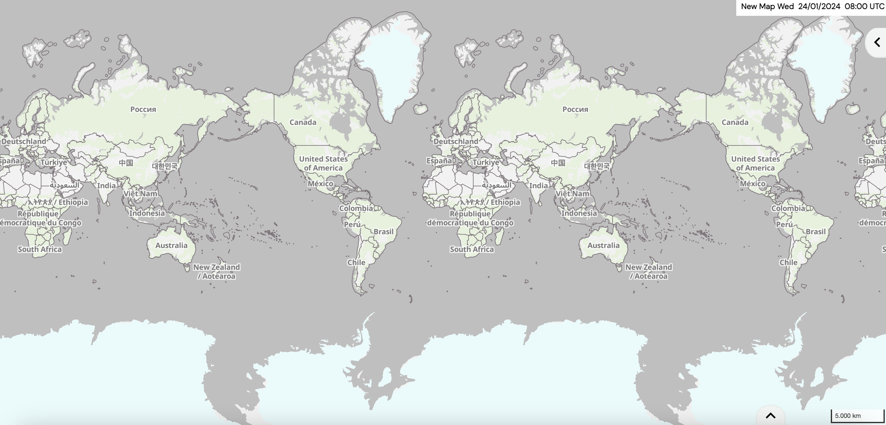
To have a closer look at a certain region, you can zoom in e.g. to Europe. Press and hold the left mouse button to change the map extent and scrolling in and out controls the level of zooming into the map.

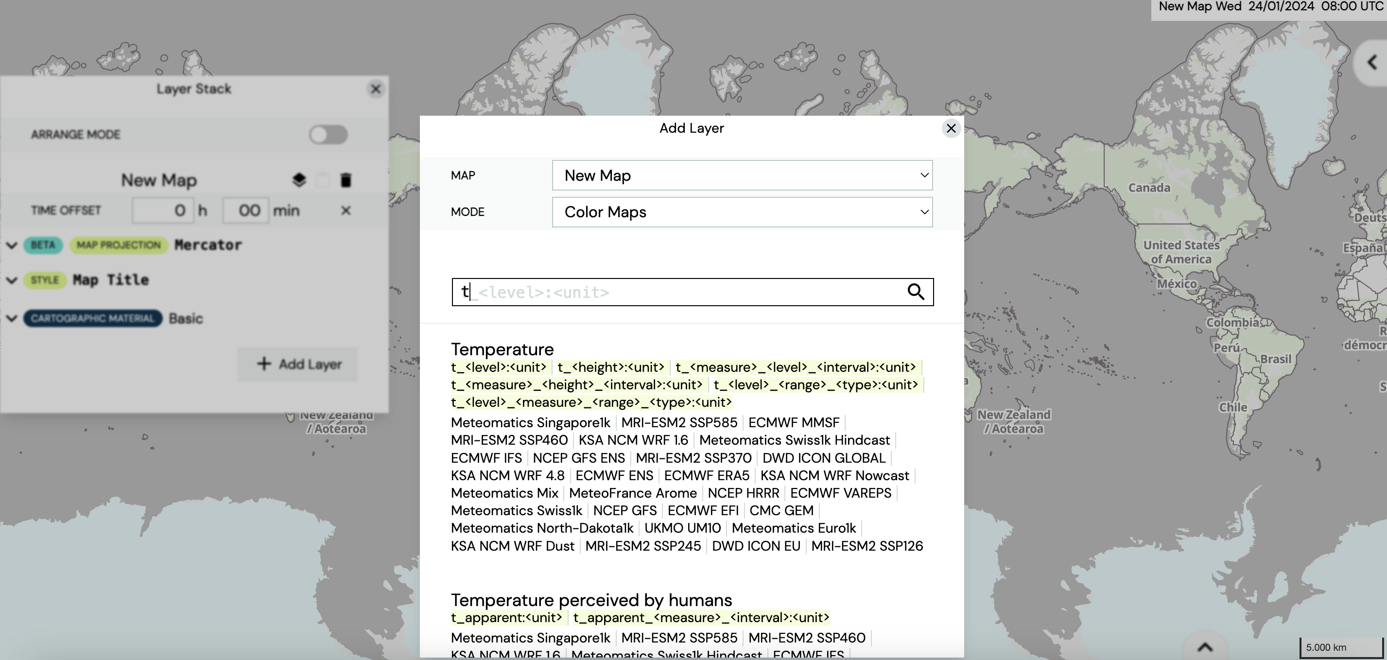
In a next step, select the desired parameters. Click on the Layer Stack Button and select the "Add Layer"-option.

A new window opens after clicking the "Add Layer" button. Select ”Color Maps” as ”MODE” and type ”t” in the ”Search for weather parameters”. Click on ”Temperature” at the very top of the suggested parameters.

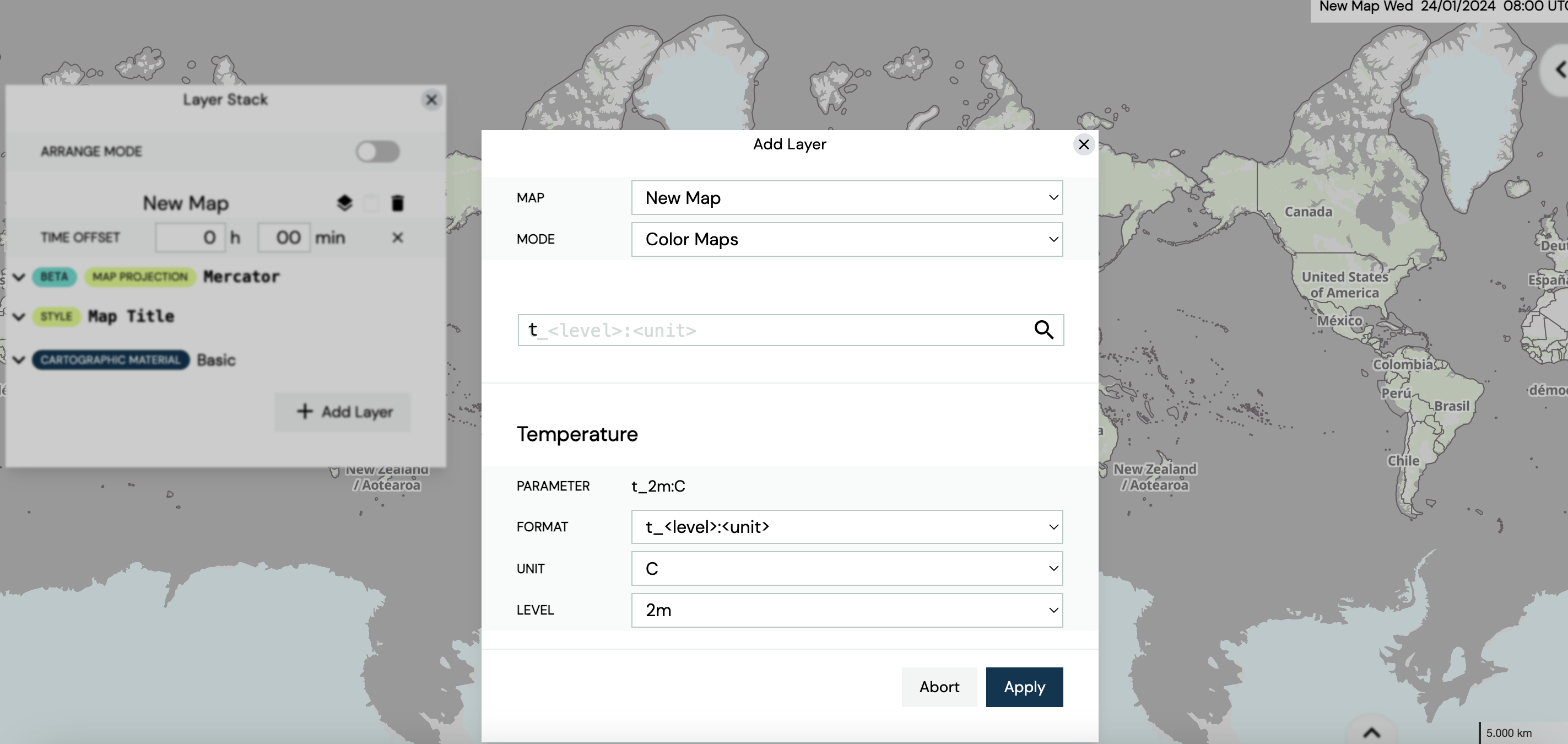
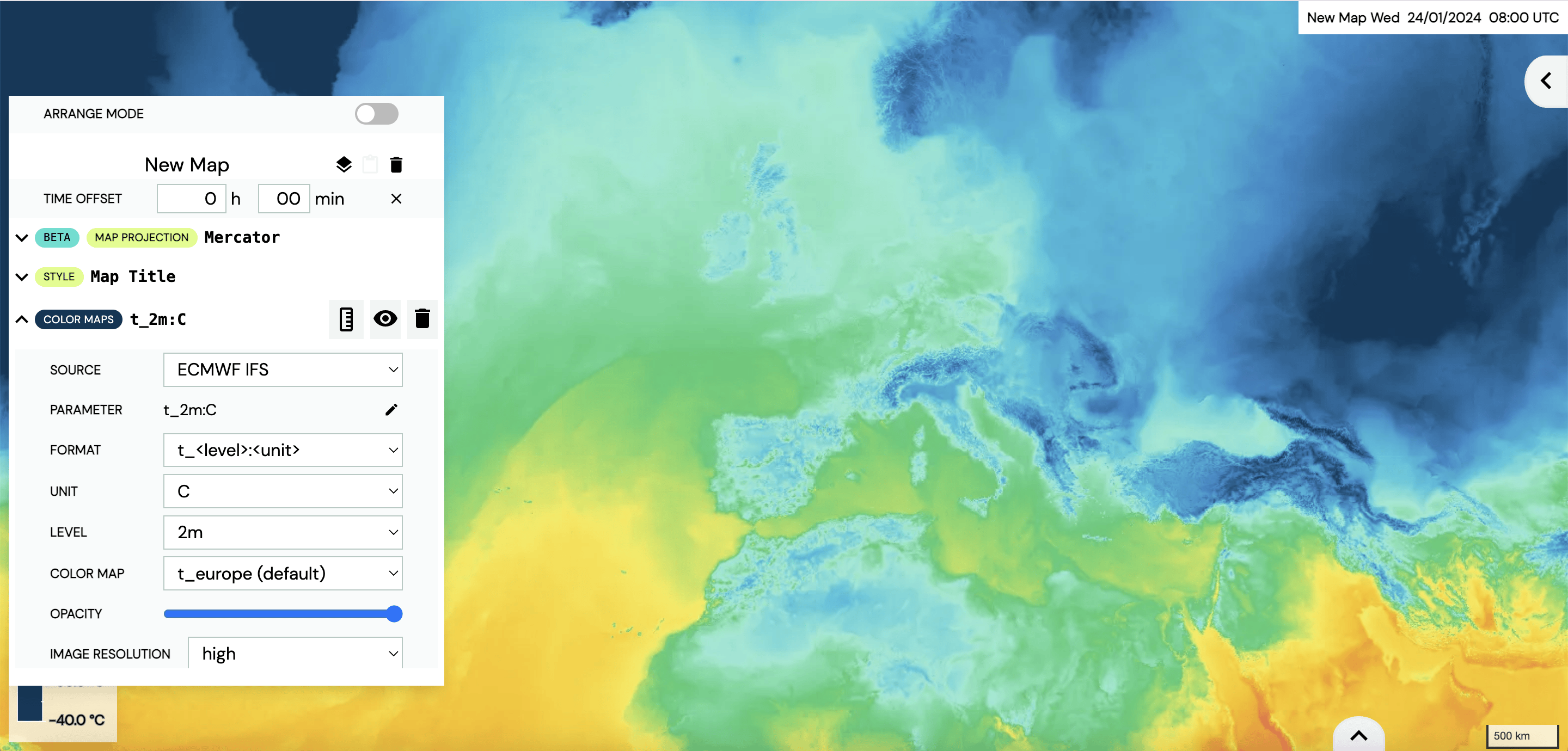
Now, you can specify the parameter properties (format, unit and level). In this example, we choose ”t_<level>:<unit>” as format, ”C” as unit and ”2m” as level to get the temperature 2 meters above the ground in °Celsius.

If desired, the user can now change the preferences of the temperature by clicking on ”COLOR MAPS t_2m:C” on the Layer Stack (see section Colour Maps). In this example, we change the ”SOURCE” to ”ECMWF IFS” and the ”OPACITY” to 100% (move the slider to the right hand side). For the rest, we keep the default values.

The medium cloud cover is the next parameter that we want to add to our map. Click on ”Add Layer” on the bottom right of the Layer Stack. Select ”Color Maps” as ”MODE” and type ”me” in the ”Search for weather parameters”. Click on ”Medium cloud cover” at the very top of the suggested parameters.

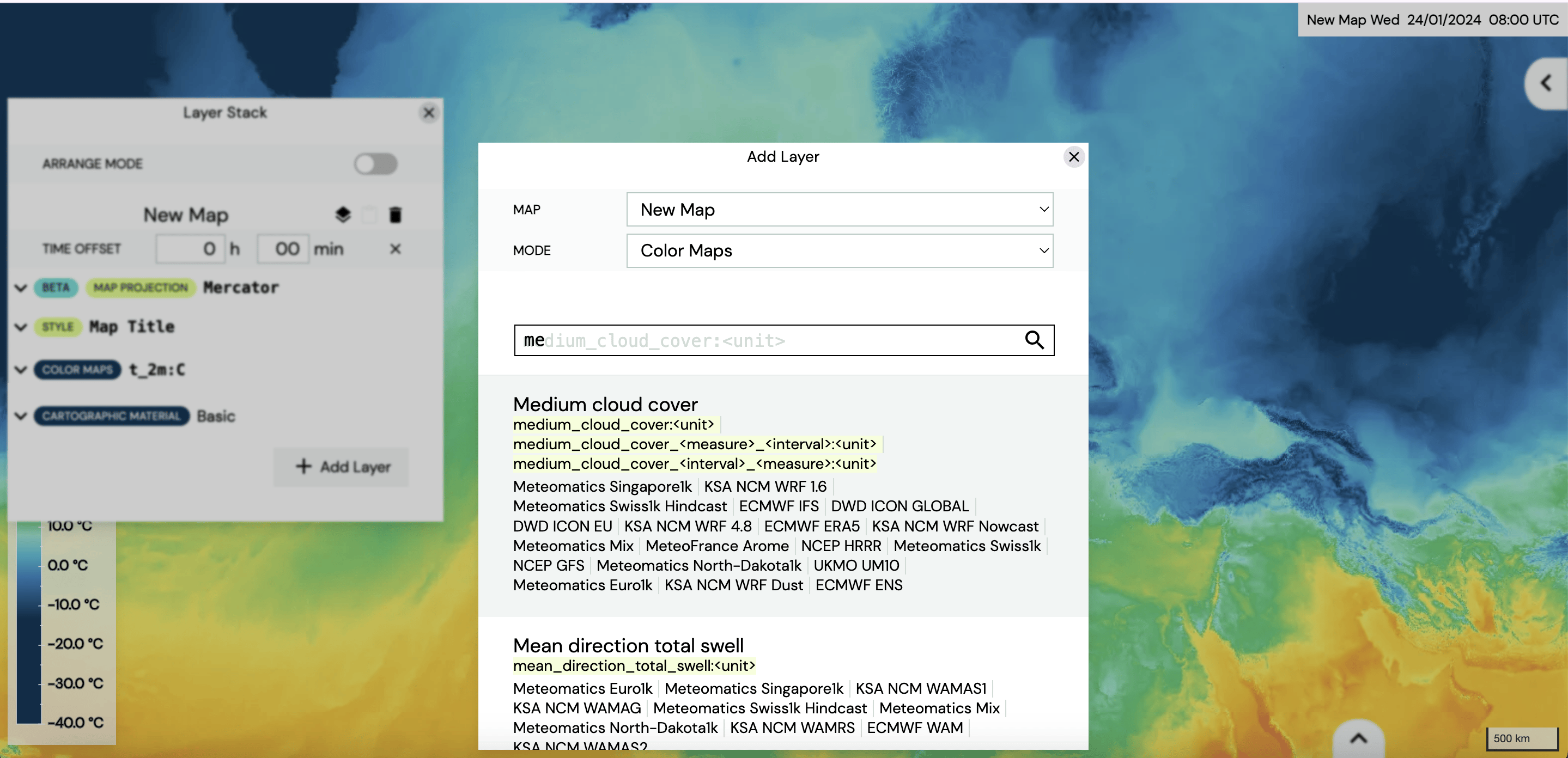
Specify the parameter properties (format and unit). In this example, we choose ”medium_cloud_cover:<unit>” as format and ”octas” as unit.

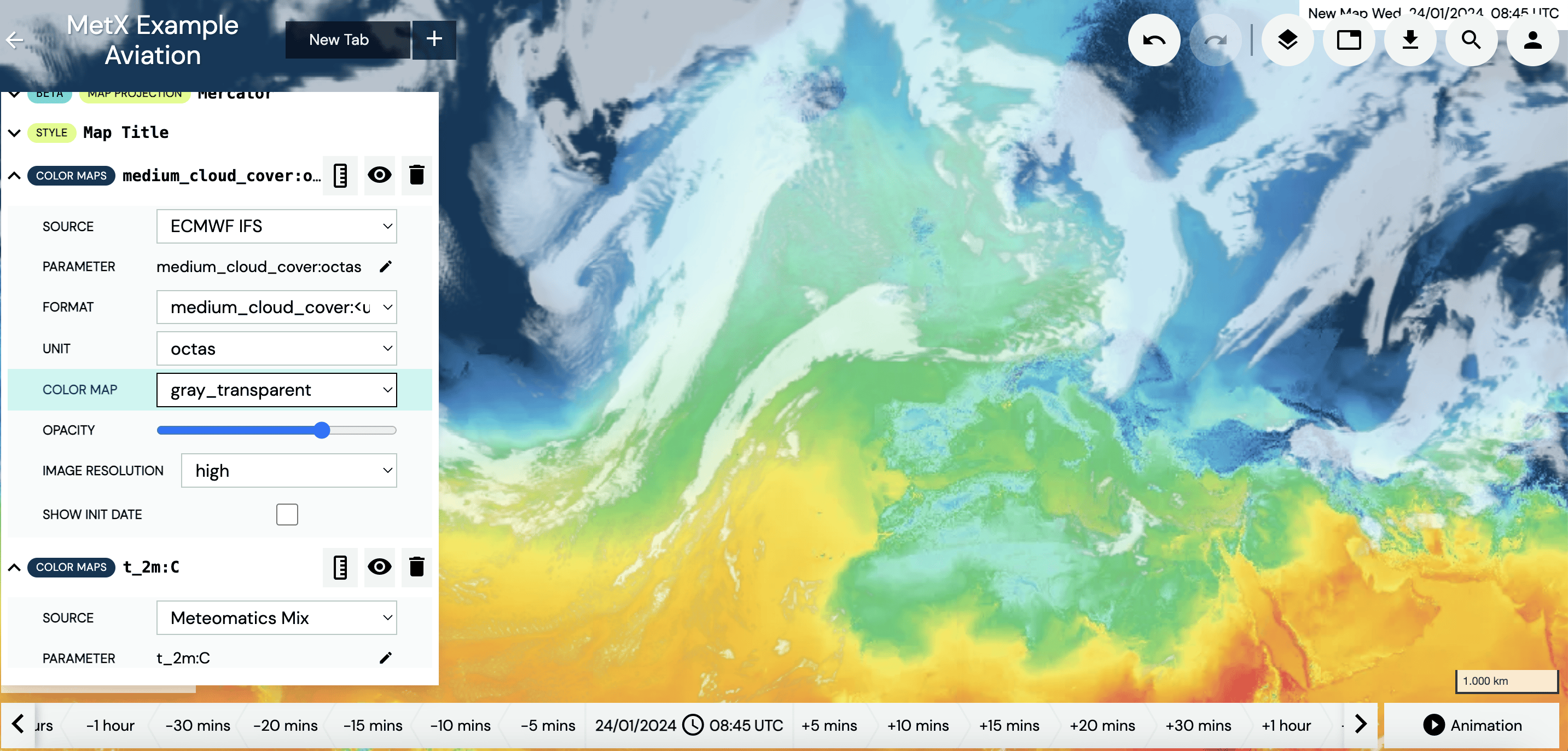
Click on ”Apply” so that the medium cloud cover in octas is displayed on the map. Now, the preferences of the medium cloud cover can be changed by clicking on ”COLOR MAPS medium_cloud_cover:octas” on the Layer Stack. In this example, we change the ”SOURCE” to ”ECMWF IFS” and the ”COLOR MAP” to ”gray_transparent”. For the rest, we keep the default values.

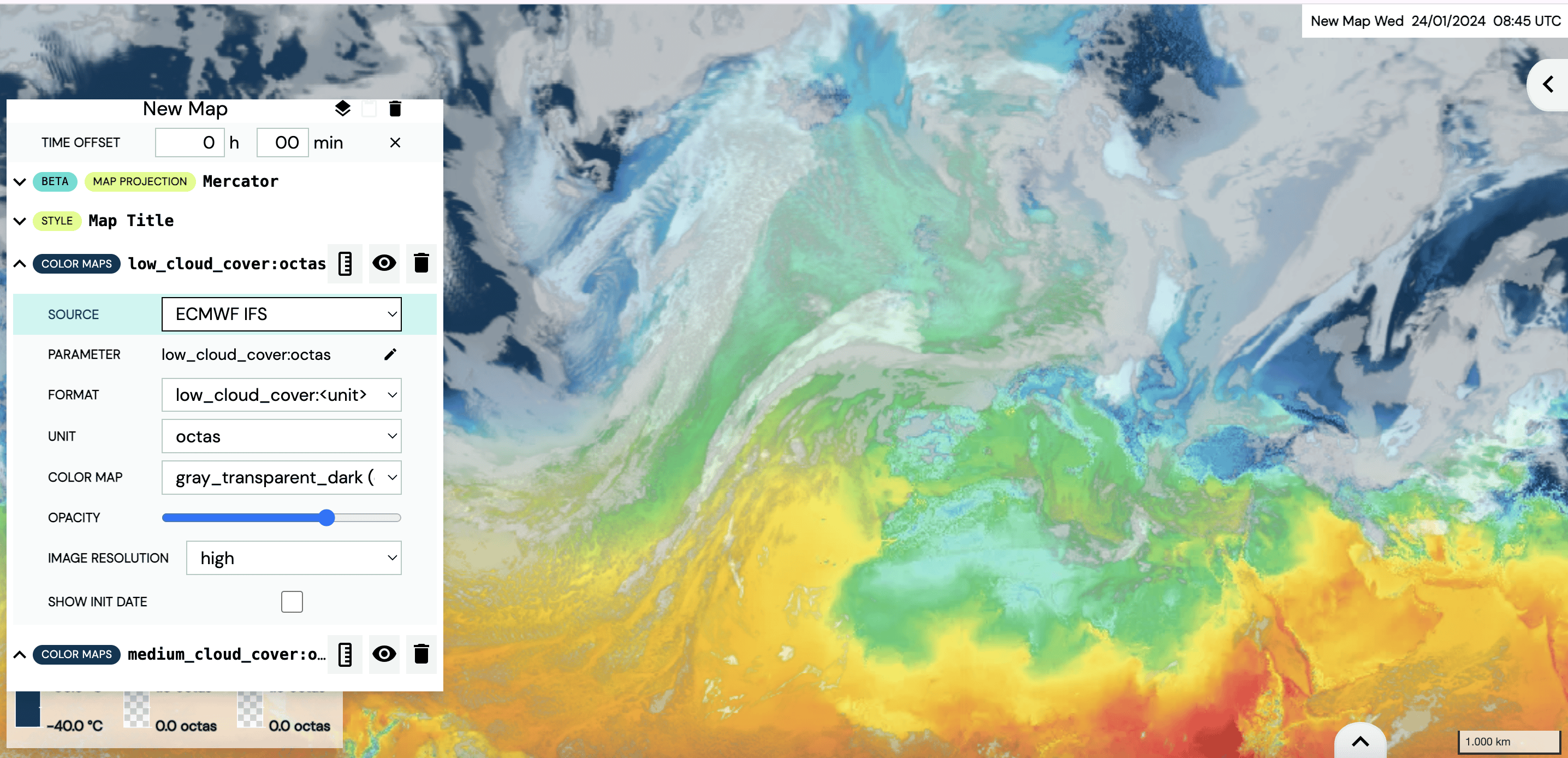
The next parameter that we want to add is the low cloud cover. Again, click on ”Add Layer” on the bot- tom right of the Layer Stack. Select ”Color Maps” as ”MODE” and type ”lo” in the ”Search for weather parameters”. Click on ”Low cloud cover” at the very top of the suggested parameters.

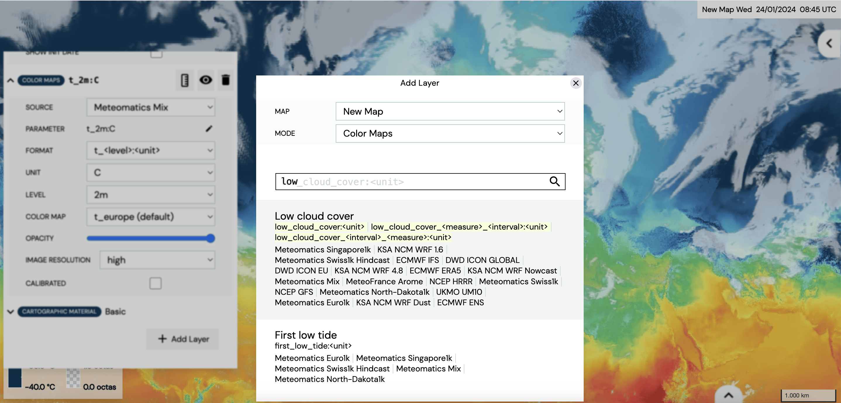
Click on ”Apply” so that the low cloud cover in octas is displayed on the map. Now, the preferences of the low cloud cover can be changed by clicking on ”COLOR MAPS low_cloud_cover:octas” on the Layer Stack (see section Colour Maps). In this example, we change the ”SOURCE” to ”ECMWF IFS” and keep for the rest the default values.

As a next parameter we add the precipitation type and intensity to the map. Click on ”Add Layer” on the bottom right of the Layer Stack. Select ”Color Maps” as ”MODE” and type ”precip” in the ”Search for weather parameters”. Scroll down and click on ”Precipitation type intensity”.

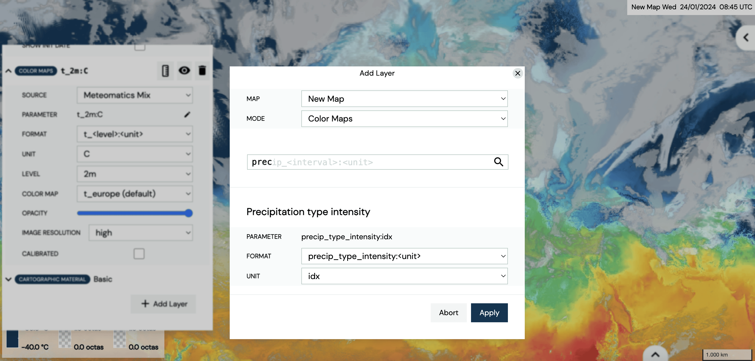
Specify the parameter properties (format, unit and interval). In this example, we choose ”precip_type_intensity_<interval>:<unit>” as format, ”idx”.

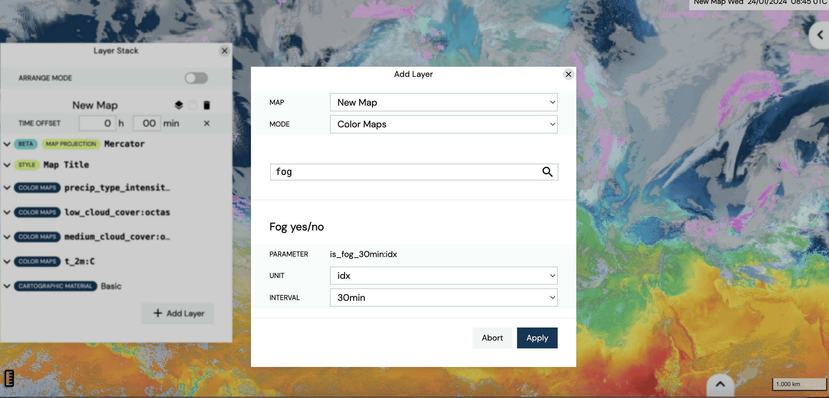
The last parameter that we add as color map on this map is the fog index. Click on ”Add Layer” on the bottom right of the Layer Stack. Select ”Color Maps” as ”MODE” and type ”fog” in the ”Search for weather parameters”. Click on ”Fog yes/no” at the very top of the suggested parameters.

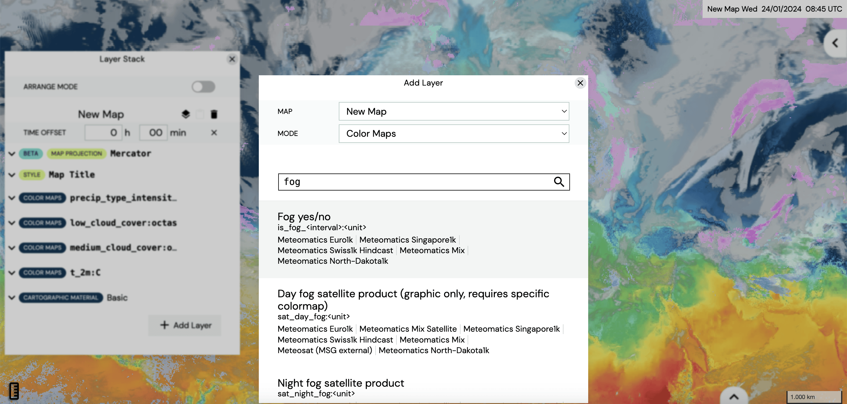
Specify the parameter properties (unit and interval). In this example, we choose ”idx” as unit and an interval of ”30min”.

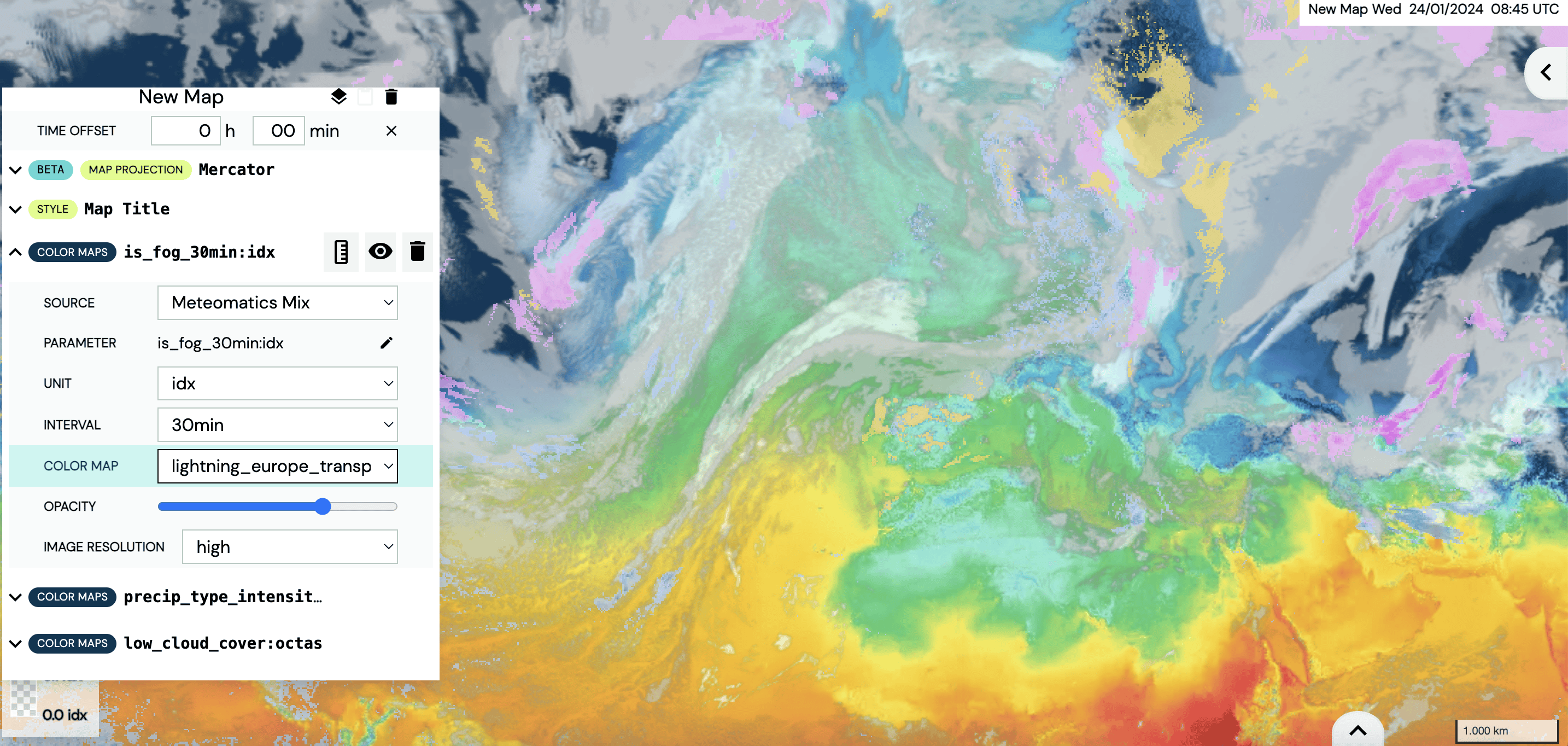
Click on ”Apply” so that the fog index is displayed on the map. Now, the preferences of the fog index can be changed by clicking on ”COLOR MAPS is_fog_30min:idx” on the Layer Stack (see section Colour Maps). In this example, we change the ”COLOR MAP” to ”lightning_europe_transparent” and the ”OPACITY” to 100% (move the slider to the right hand side). For the rest, we keep the default values.

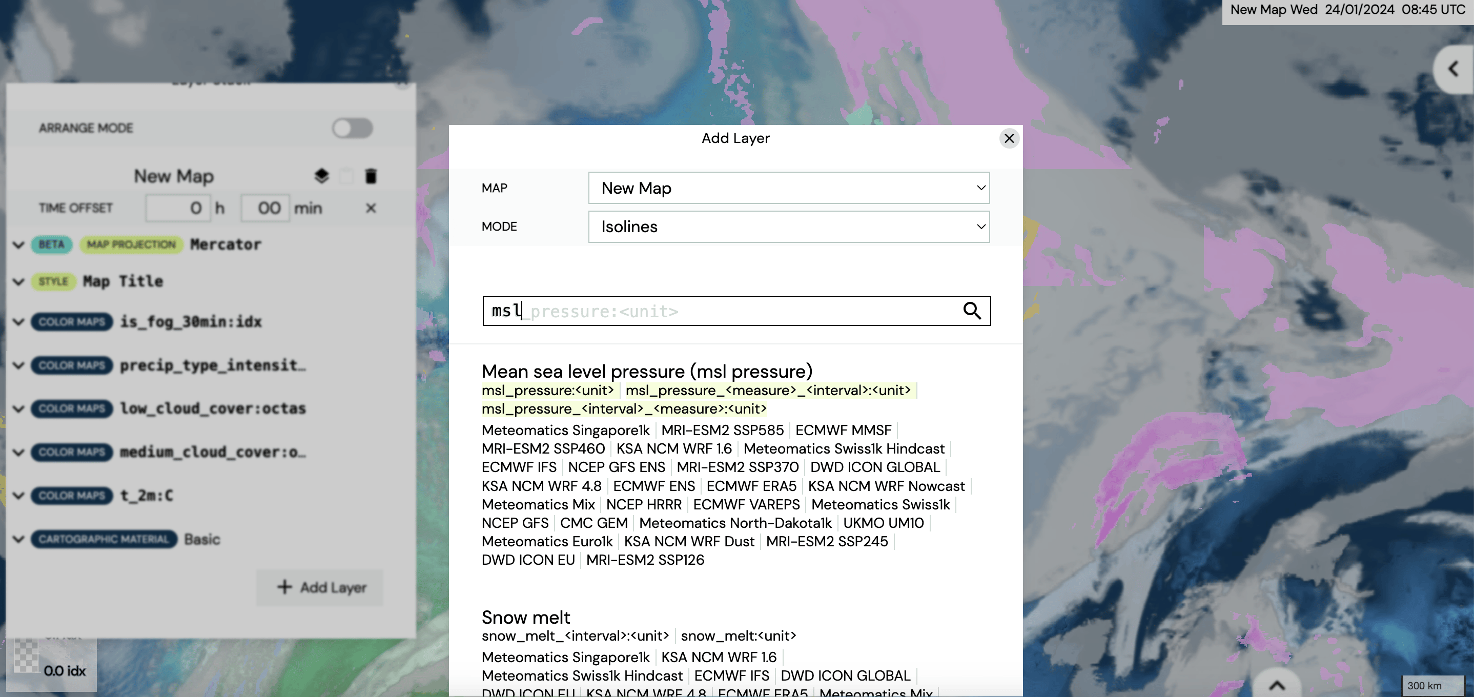
Next, we want to insert the isolines of the mean sea level pressure. Click on the ”Add Layer” button on the bottom right of the Layer Stack. Select ”Isolines” as ”MODE” and type ”msl” in the ”Search for weather parameters” box to add pressure isolines to the map (see section Isolines). Select the parameter ”Mean sea level pressure” at the very top by clicking on it and specify afterwards the parameter properties (format and unit).

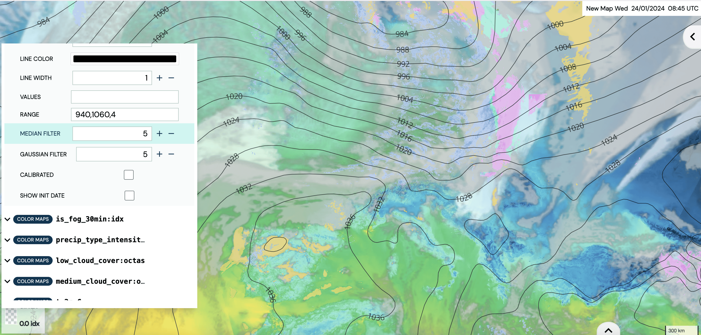
To change the preferences for the mean sea level parameter, click on the Layer Stack on ”ISOLINES msl_pressure:hPa”. In this example, we change the ”SOURCE” to ”ECMWF IFS”. Furthermore, we would like to change the displayed range and spacing of the isolines. Type the minimum, maximum and the step in the ”RANGE” box. We choose a minimum of 940 hPa, a maximum of 1060 hPa and a step of 4 hPa. In addition, we set the ”MEDIAN FILTER” as well as the ”GAUSSIAN FILTER” to 5 (see also section Isolines).

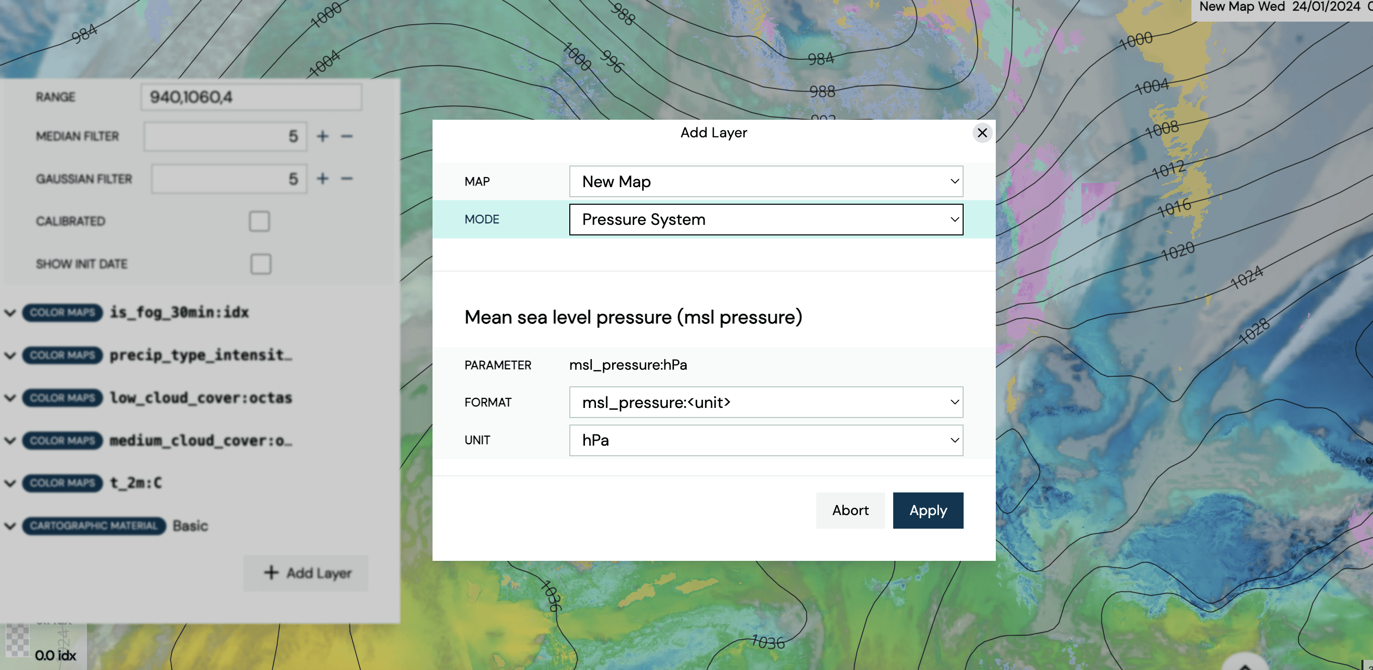
To add the symbols ”L” and ”H” in the center of the pressure systems, click on the ”Add Layer” button on the bottom right of the Layer Stack. Select ”Pressure System” as ”MODE” and specify the format and unit. In this example, we choose ”msl_pressure:<unit>” and the unit ”hPa”. Click on ”Apply” to add the symbols to the map (see also section Pressure System).

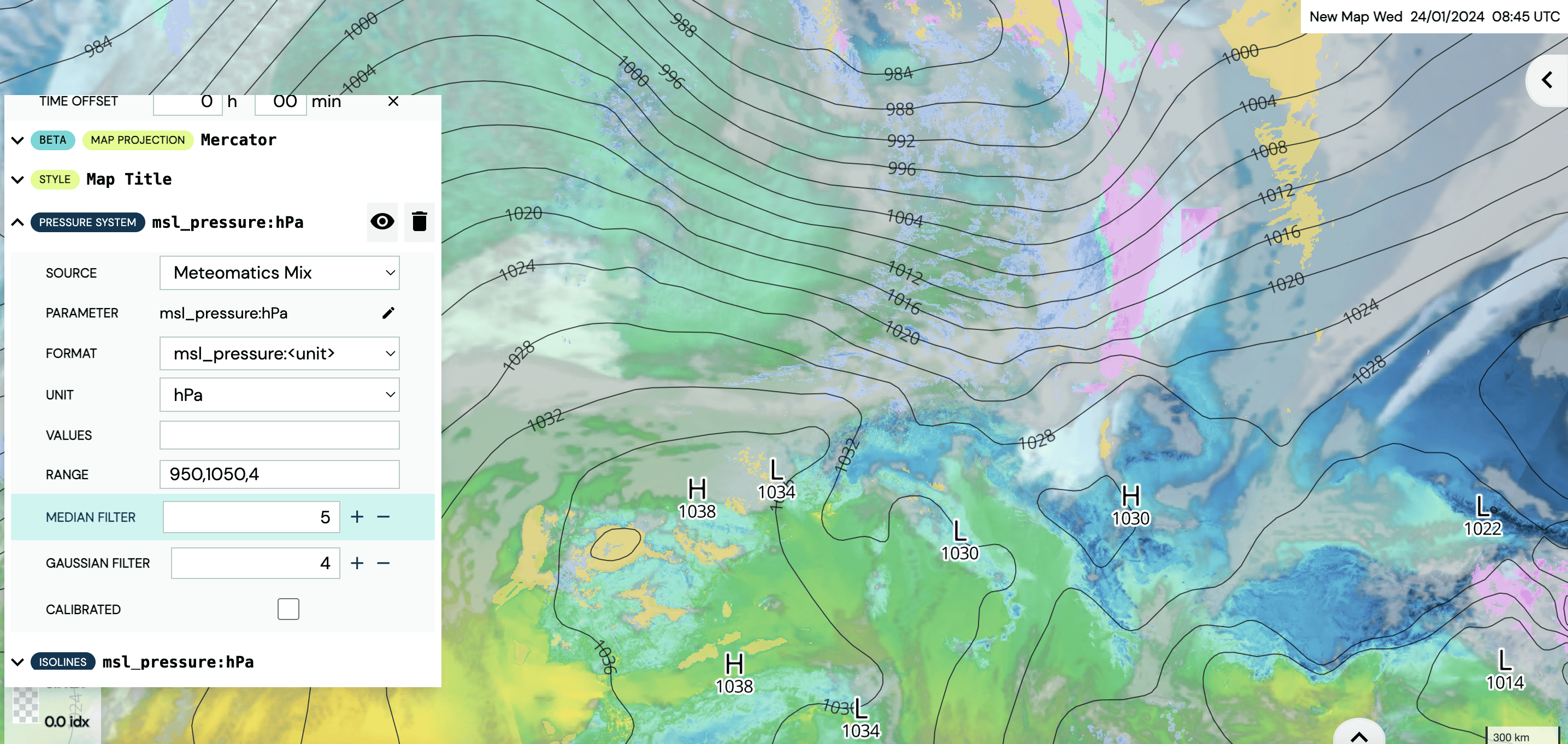
Change the preferences of the pressure system by clicking on ”PRESSURE SYSTEM msl_pressure:hPa” on the Layer Stack (see section Pressure System). In this example, we change the ”MEDIAN FILTER” and set it to 5 and change the ”GAUSSIAN FILTER” and set it to 4.

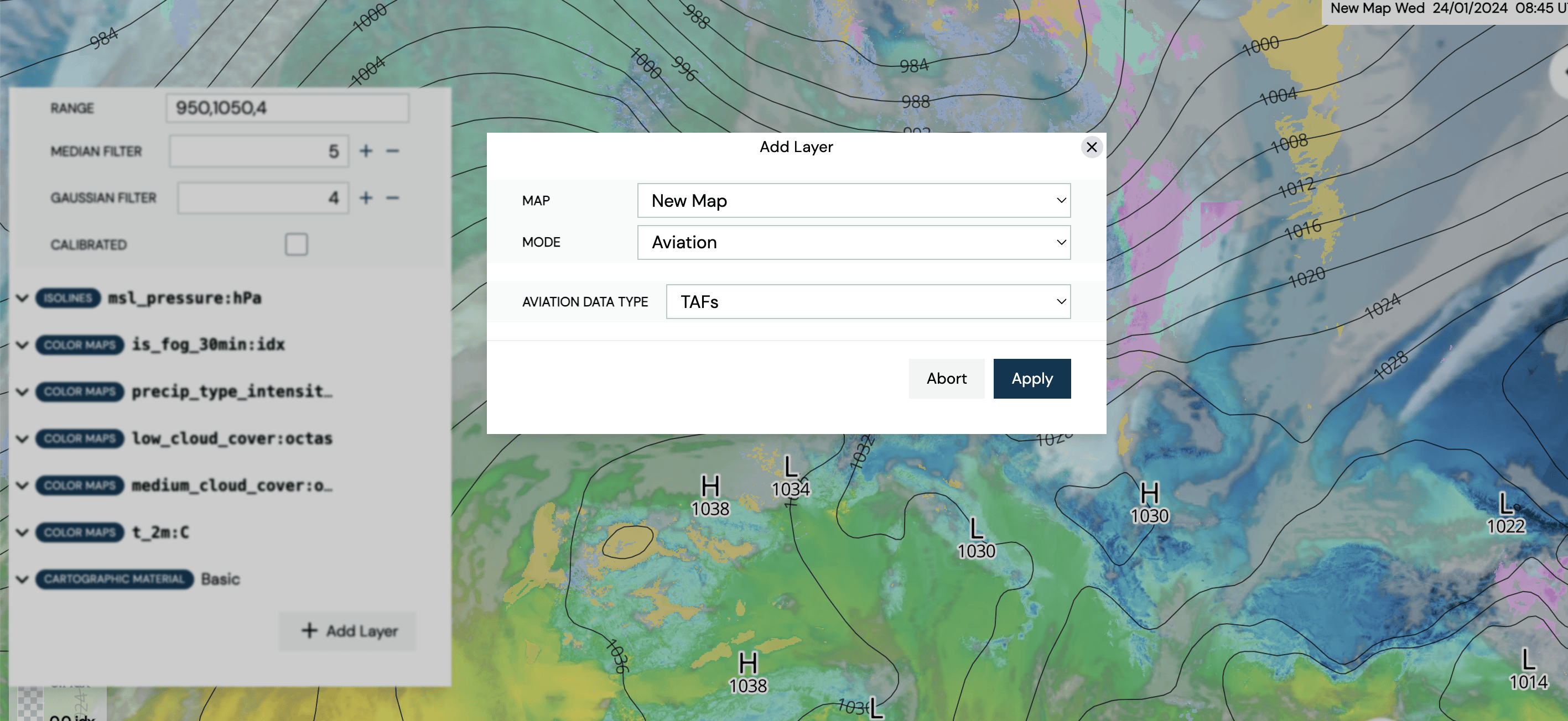
Finally, you can add typical aviation-related data such as (international) SIGMETs, METARs, TAFs, and AIREPs (see section Aviation).
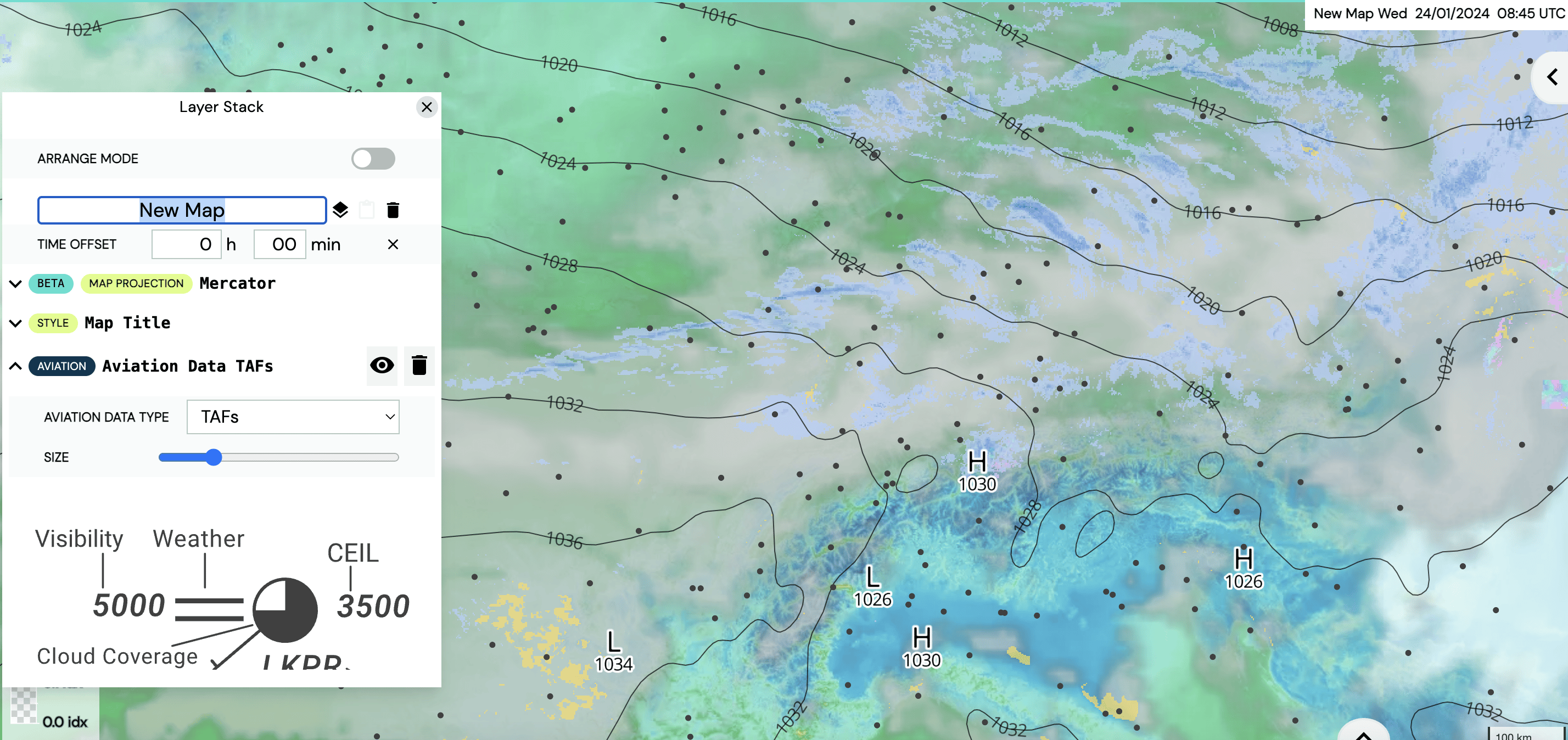
Click the ”Add Layer” button on the bottom right of the Layer Stack. Select ”Aviation” in the ”MODE” section and ”TAFs” in the ”AVIATION DATA TYPE” section. Click the ”Apply” button so that the TAFs are displayed on your map.

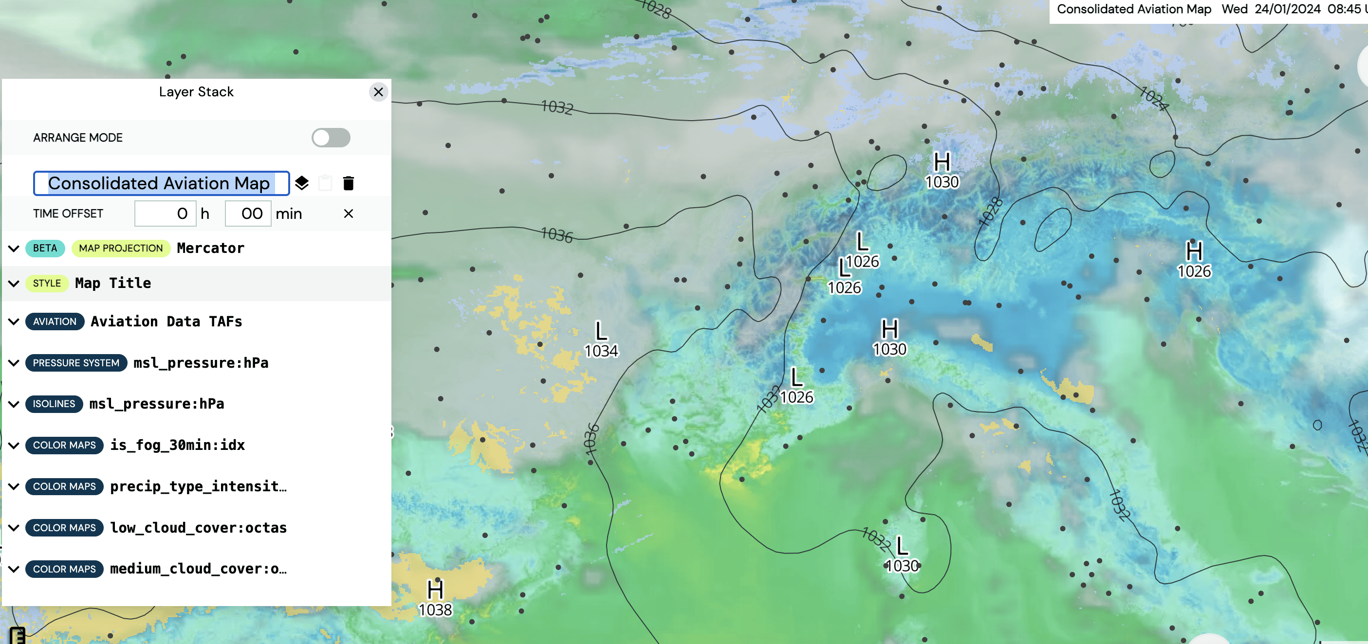
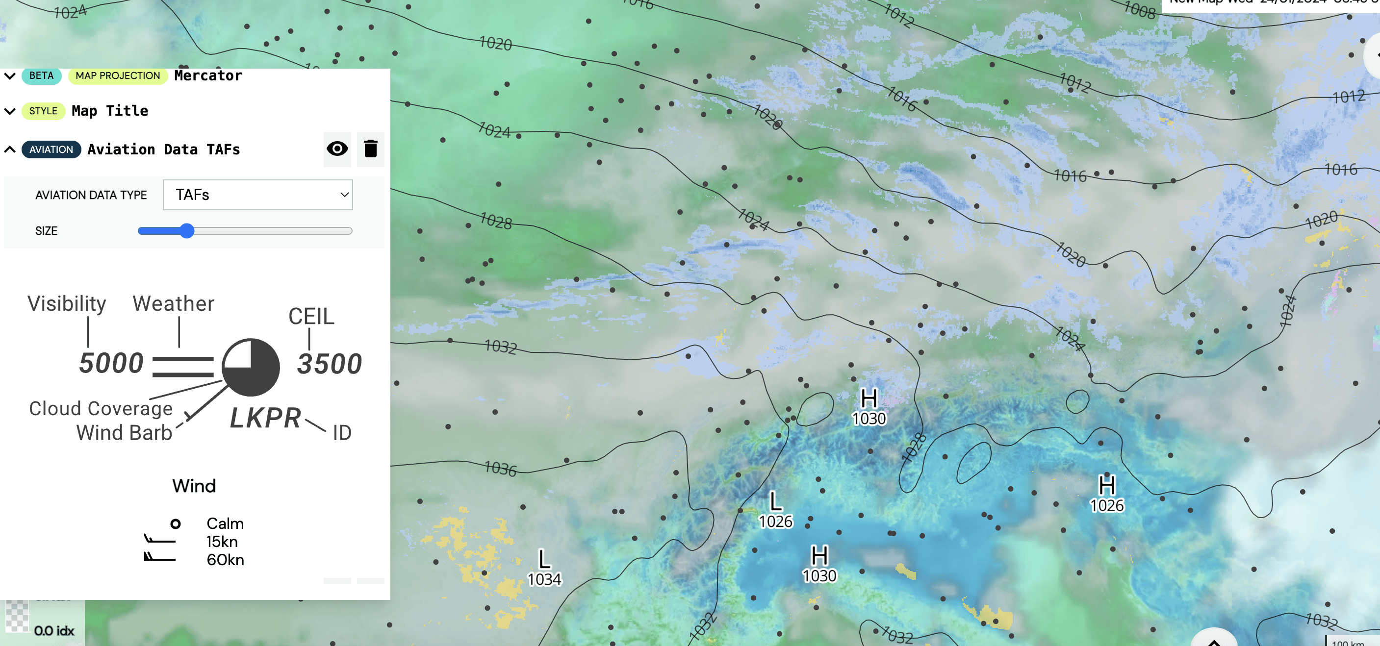
If it is wished, the user can change the preferences of the TAFs by clicking on ”AVIATION Aviation Data TAFs” on the Layer Stack (see section Aviation). In this example, we keep the default setting. Also, you can see there the legend of the symbols that are displayed on the map.

As a last step, we change the title of the map by clicking on ”New Map” on the Layer Stack and typing e.g. ”Consolidated Aviation Map” in the box. Click the ”STYLE Map Title” on the Layer Stack to adapt the design of the title (see section Map title design). In this example, we keep the default setting.

As a last step, we change the title of the map by clicking on ”New Map” on the Layer Stack and typing e.g. ”Consolidated Aviation Map” in the box. Click the ”STYLE Map Title” on the Layer Stack to adapt the design of the title (see section Map title design). In this example, we keep the default setting.